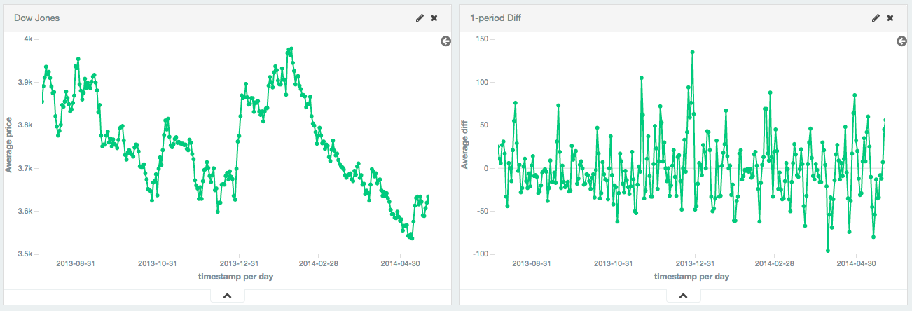
Serial differencing is a technique where values in a time series are subtracted from itself at different time lags or periods. For example, the datapoint f(x) = f(xt) - f(xt-n), where n is the period being used.
A period of 1 is equivalent to a derivative with no time normalization: it is simply the change from one point to the next. Single periods are useful for removing constant, linear trends.
Single periods are also useful for transforming data into a stationary series. In this example, the Dow Jones is plotted over ~250 days. The raw data is not stationary, which would make it difficult to use with some techniques.
By calculating the first-difference, we de-trend the data (e.g. remove a constant, linear trend). We can see that the data becomes a stationary series (e.g. the first difference is randomly distributed around zero, and doesn’t seem to exhibit any pattern/behavior). The transformation reveals that the dataset is following a random-walk; the value is the previous value +/- a random amount. This insight allows selection of further tools for analysis.
Larger periods can be used to remove seasonal / cyclic behavior. In this example, a population of lemmings was synthetically generated with a sine wave + constant linear trend + random noise. The sine wave has a period of 30 days.
The first-difference removes the constant trend, leaving just a sine wave. The 30th-difference is then applied to the first-difference to remove the cyclic behavior, leaving a stationary series which is amenable to other analysis.
A serial_diff aggregation looks like this in isolation:
{
    "serial_diff": {
        "buckets_path": "the_sum",
        "lag": "7"
    }
}
Table 30. serial_diff Parameters
| Parameter Name | Description | Required | Default Value |
|---|---|---|---|
| Path to the metric of interest (see | Required | |
| The historical bucket to subtract from the current value. E.g. a lag of 7 will subtract the current value from the value 7 buckets ago. Must be a positive, non-zero integer | Optional |
|
| Determines what should happen when a gap in the data is encountered. | Optional |
|
| Format to apply to the output value of this aggregation | Optional |
|
serial_diff aggregations must be embedded inside of a histogram or date_histogram aggregation:
POST /_search
{
"size": 0,
"aggs": {
"my_date_histo": {  "date_histogram": {
"field": "timestamp",
"interval": "day"
},
"aggs": {
"the_sum": {
"sum": {
"field": "lemmings"
  }
},
"thirtieth_difference": {
"serial_diff": {
}
},
"thirtieth_difference": {
"serial_diff": {  "buckets_path": "the_sum",
"lag" : 30
}
}
}
}
}
}
A | |
A | |
Finally, we specify a |
Serial differences are built by first specifying a histogram or date_histogram over a field. You can then optionally
add normal metrics, such as a sum, inside of that histogram. Finally, the serial_diff is embedded inside the histogram.
The buckets_path parameter is then used to "point" at one of the sibling metrics inside of the histogram (see
buckets_path Syntax for a description of the syntax for buckets_path.

