Optimization tips

... durch planmässiges Tattonieren.

[... through systematic, palpable experimentation.]

—Johann Karl Friedrich Gauss [asked how he came upon his theorems]

On this chapter, you will get deeper knowledge of PyTables internals. PyTables has many tunable features so that you can improve the performance of your application. If you are planning to deal with really large data, you should read carefully this section in order to learn how to get an important efficiency boost for your code. But if your datasets are small (say, up to 10 MB) or your number of nodes is contained (up to 1000), you should not worry about that as the default parameters in PyTables are already tuned for those sizes (although you may want to adjust them further anyway). At any rate, reading this chapter will help you in your life with PyTables.

Understanding chunking

The underlying HDF5 library that is used by PyTables allows for certain datasets (the so-called chunked datasets) to take the data in bunches of a certain length, named chunks, and write them on disk as a whole, i.e. the HDF5 library treats chunks as atomic objects and disk I/O is always made in terms of complete chunks. This allows data filters to be defined by the application to perform tasks such as compression, encryption, check-summing, etc. on entire chunks.

HDF5 keeps a B-tree in memory that is used to map chunk structures on disk. The more chunks that are allocated for a dataset the larger the B-tree. Large B-trees take memory and cause file storage overhead as well as more disk I/O and higher contention forthe metadata cache. Consequently, it’s important to balance between memory and I/O overhead (small B-trees) and time to access data (big B-trees).

In the next couple of sections, you will discover how to inform PyTables about the expected size of your datasets for allowing a sensible computation of the chunk sizes. Also, you will be presented some experiments so that you can get a feeling on the consequences of manually specifying the chunk size. Although doing this latter is only reserved to experienced people, these benchmarks may allow you to understand more deeply the chunk size implications and let you quickly start with the fine-tuning of this important parameter.

Informing PyTables about expected number of rows in tables or arrays

PyTables can determine a sensible chunk size to your dataset size if you helps it by providing an estimation of the final number of rows for an extensible leaf [1]. You should provide this information at leaf creation time by passing this value to the expectedrows argument of the File.create_table() method or File.create_earray() method (see The EArray class). For VLArray leaves, you must pass the expected size in MBytes by using the argument expectedsizein MB of File.create_vlarray() (see The VLArray class) instead.

When your leaf size is bigger than 10 MB (take this figure only as a reference, not strictly), by providing this guess you will be optimizing the access to your data. When the table or array size is larger than, say 100MB, you are strongly suggested to provide such a guess; failing to do that may cause your application to do very slow I/O operations and to demand huge amounts of memory. You have been warned!

Fine-tuning the chunksize

Warning

This section is mostly meant for experts. If you are a beginner, you must know that setting manually the chunksize is a potentially dangerous action.

Most of the time, informing PyTables about the extent of your dataset is enough. However, for more sophisticated applications, when one has special requirements for doing the I/O or when dealing with really large datasets, you should really understand the implications of the chunk size in order to be able to find the best value for your own application.

You can specify the chunksize for every chunked dataset in PyTables by passing the chunkshape argument to the corresponding constructors. It is important to point out that chunkshape is not exactly the same thing than a chunksize; in fact, the chunksize of a dataset can be computed multiplying all the dimensions of the chunkshape among them and multiplying the outcome by the size of the atom.

We are going to describe a series of experiments where an EArray of 15 GB is written with different chunksizes, and then it is accessed in both sequential (i.e. first element 0, then element 1 and so on and so forth until the data is exhausted) and random mode (i.e. single elements are read randomly all through the dataset). These benchmarks have been carried out with PyTables 2.1 on a machine with an Intel Core2 processor @ 3 GHz and a RAID-0 made of two SATA disks spinning at 7200 RPM, and using GNU/Linux with an XFS filesystem. The script used for the benchmarks is available in bench/optimal-chunksize.py.

In figures Figure 1, Figure 2, Figure 3 and Figure 4, you can see how the chunksize affects different aspects, like creation time, file sizes, sequential read time and random read time. So, if you properly inform PyTables about the extent of your datasets, you will get an automatic chunksize value (256 KB in this case) that is pretty optimal for most of uses. However, if what you want is, for example, optimize the creation time when using the Zlib compressor, you may want to reduce the chunksize to 32 KB (see Figure 1). Or, if your goal is to optimize the sequential access time for an dataset compressed with Blosc, you may want to increase the chunksize to 512 KB (see Figure 3).

You will notice that, by manually specifying the chunksize of a leave you will not normally get a drastic increase in performance, but at least, you have the opportunity to fine-tune such an important parameter for improve performance.

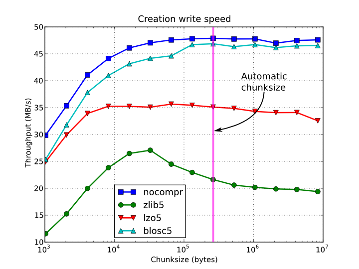
Figure 1. Creation time per element for a 15 GB EArray and different chunksizes.

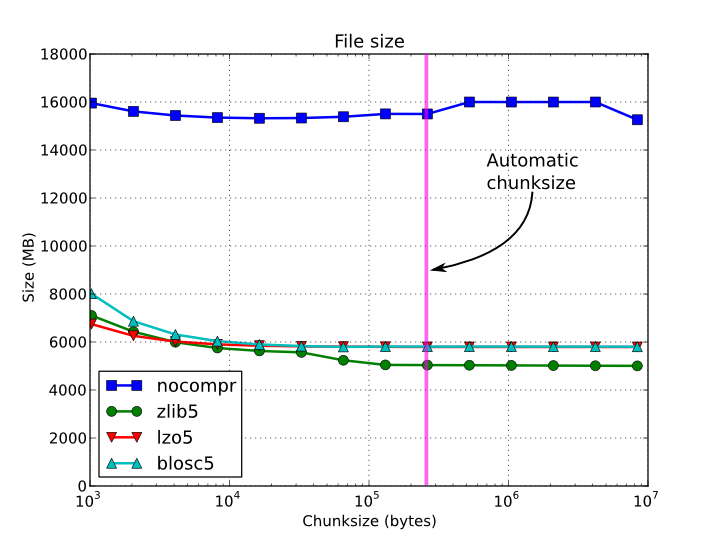
Figure 2. File sizes for a 15 GB EArray and different chunksizes.

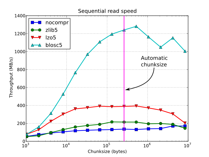
Figure 3. Sequential access time per element for a 15 GB EArray and different chunksizes.

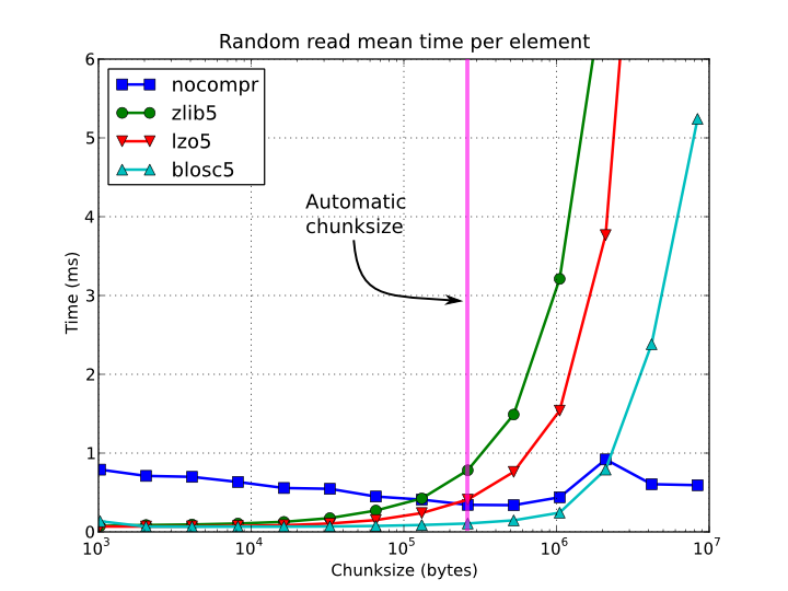
Figure 4. Random access time per element for a 15 GB EArray and different chunksizes.

Finally, it is worth noting that adjusting the chunksize can be specially important if you want to access your dataset by blocks of certain dimensions. In this case, it is normally a good idea to set your chunkshape to be the same than these dimensions; you only have to be careful to not end with a too small or too large chunksize. As always, experimenting prior to pass your application into production is your best ally.

Accelerating your searches

Note

Many of the explanations and plots in this section and the forthcoming ones still need to be updated to include Blosc (see [BLOSC]), the new and powerful compressor added in PyTables 2.2 series. You should expect it to be the fastest compressor among all the described here, and its use is strongly recommended whenever you need extreme speed and not a very high compression ratio.

Searching in tables is one of the most common and time consuming operations that a typical user faces in the process of mining through his data. Being able to perform queries as fast as possible will allow more opportunities for finding the desired information quicker and also allows to deal with larger datasets.

PyTables offers many sort of techniques so as to speed-up the search process as much as possible and, in order to give you hints to use them based, a series of benchmarks have been designed and carried out. All the results presented in this section have been obtained with synthetic, random data and using PyTables 2.1. Also, the tests have been conducted on a machine with an Intel Core2 (64-bit) @ 3 GHz processor with RAID-0 disk storage (made of four spinning disks @ 7200 RPM), using GNU/Linux with an XFS filesystem. The script used for the benchmarks is available in bench/indexed_search.py. As your data, queries and platform may be totally different for your case, take this just as a guide because your mileage may vary (and will vary).

In order to be able to play with tables with a number of rows as large as possible, the record size has been chosen to be rather small (24 bytes). Here it is its definition:

class Record(tables.IsDescription):
    col1 = tables.Int32Col()
    col2 = tables.Int32Col()
    col3 = tables.Float64Col()
    col4 = tables.Float64Col()

In the next sections, we will be optimizing the times for a relatively complex query like this:

result = [row['col2'] for row in table if (
          ((row['col4'] >= lim1 and row['col4'] < lim2) or
          ((row['col2'] > lim3 and row['col2'] < lim4])) and
          ((row['col1']+3.1*row['col2']+row['col3']*row['col4']) > lim5)
          )]

(for future reference, we will call this sort of queries regular queries). So, if you want to see how to greatly improve the time taken to run queries like this, keep reading.

In-kernel searches

PyTables provides a way to accelerate data selections inside of a single table, through the use of the Table methods - querying iterator and related query methods. This mode of selecting data is called in-kernel. Let’s see an example of an in-kernel query based on the regular one mentioned above:

result = [row['col2'] for row in table.where(
            '''(((col4 >= lim1) & (col4 < lim2)) |
               ((col2 > lim3) & (col2 < lim4)) &
               ((col1+3.1*col2+col3*col4) > lim5))''')]

This simple change of mode selection can improve search times quite a lot and actually make PyTables very competitive when compared against typical relational databases as you can see in Figure 5 and Figure 6.

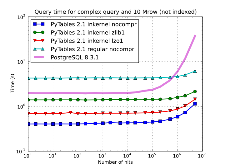
Figure 5. Times for non-indexed complex queries in a small table with 10 millions of rows: the data fits in memory.

By looking at Figure 5 you can see how in the case that table data fits easily in memory, in-kernel searches on uncompressed tables are generally much faster (10x) than standard queries as well as PostgreSQL (5x). Regarding compression, we can see how Zlib compressor actually slows down the performance of in-kernel queries by a factor 3.5x; however, it remains faster than PostgreSQL (40%). On his hand, LZO compressor only decreases the performance by a 75% with respect to uncompressed in-kernel queries and is still a lot faster than PostgreSQL (3x). Finally, one can observe that, for low selectivity queries (large number of hits), PostgreSQL performance degrades quite steadily, while in PyTables this slow down rate is significantly smaller. The reason of this behaviour is not entirely clear to the authors, but the fact is clearly reproducible in our benchmarks.

But, why in-kernel queries are so fast when compared with regular ones?. The answer is that in regular selection mode the data for all the rows in table has to be brought into Python space so as to evaluate the condition and decide if the corresponding field should be added to the result list. On the contrary, in the in-kernel mode, the condition is passed to the PyTables kernel (hence the name), written in C, and evaluated there at full C speed (with the help of the integrated Numexpr package, see [NUMEXPR]), so that the only values that are brought to Python space are the rows that fulfilled the condition. Hence, for selections that only have a relatively small number of hits (compared with the total amount of rows), the savings are very large. It is also interesting to note the fact that, although for queries with a large number of hits the speed-up is not as high, it is still very important.

On the other hand, when the table is too large to fit in memory (see Figure 6), the difference in speed between regular and in-kernel is not so important, but still significant (2x). Also, and curiously enough, large tables compressed with Zlib offers slightly better performance (around 20%) than uncompressed ones; this is because the additional CPU spent by the uncompressor is compensated by the savings in terms of net I/O (one has to read less actual data from disk). However, when using the extremely fast LZO compressor, it gives a clear advantage over Zlib, and is up to 2.5x faster than not using compression at all. The reason is that LZO decompression speed is much faster than Zlib, and that allows PyTables to read the data at full disk speed (i.e. the bottleneck is in the I/O subsystem, not in the CPU). In this case the compression rate is around 2.5x, and this is why the data can be read 2.5x faster. So, in general, using the LZO compressor is the best way to ensure best reading/querying performance for out-of-core datasets (more about how compression affects performance in Compression issues).

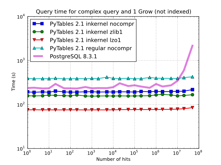
Figure 6. Times for non-indexed complex queries in a large table with 1 billion of rows: the data does not fit in memory.

Furthermore, you can mix the in-kernel and regular selection modes for evaluating arbitrarily complex conditions making use of external functions. Look at this example:

result = [ row['var2']
           for row in table.where('(var3 == "foo") & (var1 <= 20)')
           if your_function(row['var2']) ]

Here, we use an in-kernel selection to choose rows according to the values of the var3 and var1 fields. Then, we apply a regular selection to complete the query. Of course, when you mix the in-kernel and regular selection modes you should pass the most restrictive condition to the in-kernel part, i.e. to the where() iterator. In situations where it is not clear which is the most restrictive condition, you might want to experiment a bit in order to find the best combination.

However, since in-kernel condition strings allow rich expressions allowing the coexistence of multiple columns, variables, arithmetic operations and many typical functions, it is unlikely that you will be forced to use external regular selections in conditions of small to medium complexity. See Condition Syntax for more information on in-kernel condition syntax.

Indexed searches

When you need more speed than in-kernel selections can offer you, PyTables offers a third selection method, the so-called indexed mode (based on the highly efficient OPSI indexing engine ). In this mode, you have to decide which column(s) you are going to apply your selections over, and index them. Indexing is just a kind of sorting operation over a column, so that searches along such a column (or columns) will look at this sorted information by using a binary search which is much faster than the sequential search described in the previous section.

You can index the columns you want by calling the Column.create_index() method on an already created table. For example:

indexrows = table.cols.var1.create_index()
indexrows = table.cols.var2.create_index()
indexrows = table.cols.var3.create_index()

will create indexes for all var1, var2 and var3 columns.

After you have indexed a series of columns, the PyTables query optimizer will try hard to discover the usable indexes in a potentially complex expression. However, there are still places where it cannot determine that an index can be used. See below for examples where the optimizer can safely determine if an index, or series of indexes, can be used or not.

Example conditions where an index can be used:

• var1 >= “foo” (var1 is used)
• var1 >= mystr (var1 is used)
• (var1 >= “foo”) & (var4 > 0.0) (var1 is used)
• (“bar” <= var1) & (var1 < “foo”) (var1 is used)
• ((“bar” <= var1) & (var1 < “foo”)) & (var4 > 0.0) (var1 is used)
• (var1 >= “foo”) & (var3 > 10) (var1 and var3 are used)
• (var1 >= “foo”) | (var3 > 10) (var1 and var3 are used)
• ~(var1 >= “foo”) | ~(var3 > 10) (var1 and var3 are used)

Example conditions where an index can not be used:

• var4 > 0.0 (var4 is not indexed)
• var1 != 0.0 (range has two pieces)
• ~((“bar” <= var1) & (var1 < “foo”)) & (var4 > 0.0) (negation of a complex boolean expression)

Note

From PyTables 2.3 on, several indexes can be used in a single query.

Note

If you want to know for sure whether a particular query will use indexing or not (without actually running it), you are advised to use the Table.will_query_use_indexing() method.

One important aspect of the new indexing in PyTables (>= 2.3) is that it has been designed from the ground up with the goal of being capable to effectively manage very large tables. To this goal, it sports a wide spectrum of different quality levels (also called optimization levels) for its indexes so that the user can choose the best one that suits her needs (more or less size, more or less performance).

In Figure 7, you can see that the times to index columns in tables can be really short. In particular, the time to index a column with 1 billion rows (1 Gigarow) with the lowest optimization level is less than 4 minutes while indexing the same column with full optimization (so as to get a completely sorted index or CSI) requires around 1 hour. These are rather competitive figures compared with a relational database (in this case, PostgreSQL 8.3.1, which takes around 1.5 hours for getting the index done). This is because PyTables is geared towards read-only or append-only tables and takes advantage of this fact to optimize the indexes properly. On the contrary, most relational databases have to deliver decent performance in other scenarios as well (specially updates and deletions), and this fact leads not only to slower index creation times, but also to indexes taking much more space on disk, as you can see in Figure 8.

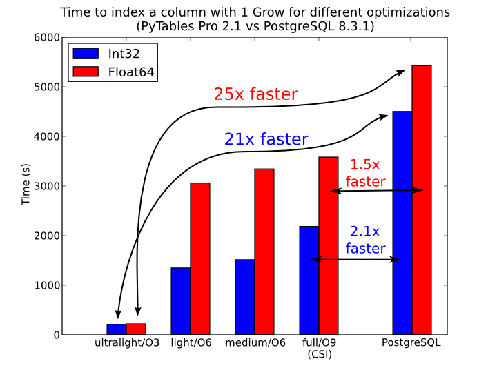
Figure 7. Times for indexing an Int32 and Float64 column.

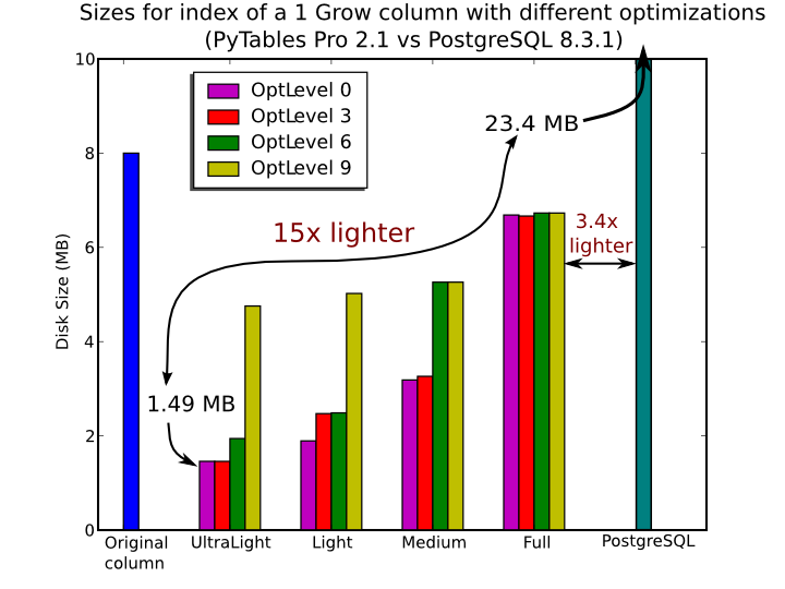
Figure 8. Sizes for an index of a Float64 column with 1 billion of rows.

The user can select the index quality by passing the desired optlevel and kind arguments to the Column.create_index() method. We can see in figures Figure 7 and Figure 8 how the different optimization levels affects index time creation and index sizes.

So, which is the effect of the different optimization levels in terms of query times? You can see that in Figure 9.

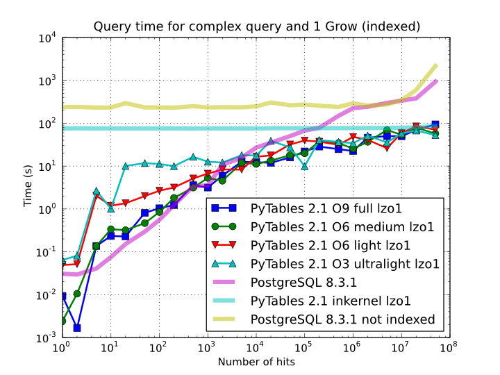
Figure 9. Times for complex queries with a cold cache (mean of 5 first random queries) for different optimization levels. Benchmark made on a machine with Intel Core2 (64-bit) @ 3 GHz processor with RAID-0 disk storage.

Of course, compression also has an effect when doing indexed queries, although not very noticeable, as can be seen in Figure 10. As you can see, the difference between using no compression and using Zlib or LZO is very little, although LZO achieves relatively better performance generally speaking.

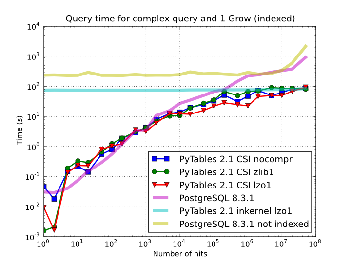
Figure 10. Times for complex queries with a cold cache (mean of 5 first random queries) for different compressors.

You can find a more complete description and benchmarks about OPSI, the indexing system of PyTables (>= 2.3) in [OPSI].

Indexing and Solid State Disks (SSD)

Lately, the long promised Solid State Disks (SSD for brevity) with decent capacities and affordable prices have finally hit the market and will probably stay in coexistence with the traditional spinning disks for the foreseeable future (separately or forming hybrid systems). SSD have many advantages over spinning disks, like much less power consumption and better throughput. But of paramount importance, specially in the context of accelerating indexed queries, is its very reduced latency during disk seeks, which is typically 100x better than traditional disks. Such a huge improvement has to have a clear impact in reducing the query times, specially when the selectivity is high (i.e. the number of hits is small).

In order to offer an estimate on the performance improvement we can expect when using a low-latency SSD instead of traditional spinning disks, the benchmark in the previous section has been repeated, but this time using a single SSD disk instead of the four spinning disks in RAID-0. The result can be seen in Figure 11. There one can see how a query in a table of 1 billion of rows with 100 hits took just 1 tenth of second when using a SSD, instead of 1 second that needed the RAID made of spinning disks. This factor of 10x of speed-up for high-selectivity queries is nothing to sneeze at, and should be kept in mind when really high performance in queries is needed. It is also interesting that using compression with LZO does have a clear advantage over when no compression is done.

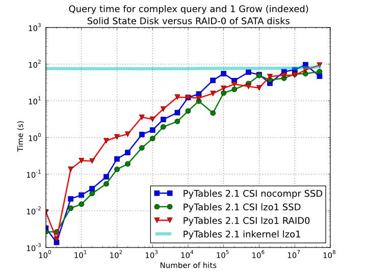
Figure 11. Times for complex queries with a cold cache (mean of 5 first random queries) for different disk storage (SSD vs spinning disks).

Finally, we should remark that SSD can’t compete with traditional spinning disks in terms of capacity as they can only provide, for a similar cost, between 1/10th and 1/50th of the size of traditional disks. It is here where the compression capabilities of PyTables can be very helpful because both tables and indexes can be compressed and the final space can be reduced by typically 2x to 5x (4x to 10x when compared with traditional relational databases). Best of all, as already mentioned, performance is not degraded when compression is used, but actually improved. So, by using PyTables and SSD you can query larger datasets that otherwise would require spinning disks when using other databases

In fact, we were unable to run the PostgreSQL benchmark in this case because the space needed exceeded the capacity of our SSD., while allowing improvements in the speed of indexed queries between 2x (for medium to low selectivity queries) and 10x (for high selectivity queries).

Achieving ultimate speed: sorted tables and beyond

Warning

Sorting a large table is a costly operation. The next procedure should only be performed when your dataset is mainly read-only and meant to be queried many times.

When querying large tables, most of the query time is spent in locating the interesting rows to be read from disk. In some occasions, you may have queries whose result depends mainly of one single column (a query with only one single condition is the trivial example), so we can guess that sorting the table by this column would lead to locate the interesting rows in a much more efficient way (because they would be mostly contiguous). We are going to confirm this guess.

For the case of the query that we have been using in the previous sections:

result = [row['col2'] for row in table.where(
            '''(((col4 >= lim1) & (col4 < lim2)) |
               ((col2 > lim3) & (col2 < lim4)) &
               ((col1+3.1*col2+col3*col4) > lim5))''')]

it is possible to determine, by analysing the data distribution and the query limits, that col4 is such a main column. So, by ordering the table by the col4 column (for example, by specifying setting the column to sort by in the sortby parameter in the Table.copy() method and re-indexing col2 and col4 afterwards, we should get much faster performance for our query. This is effectively demonstrated in Figure 12, where one can see how queries with a low to medium (up to 10000) number of hits can be done in around 1 tenth of second for a RAID-0 setup and in around 1 hundredth of second for a SSD disk. This represents up to more that 100x improvement in speed with respect to the times with unsorted tables. On the other hand, when the number of hits is large (> 1 million), the query times grow almost linearly, showing a near-perfect scalability for both RAID-0 and SSD setups (the sequential access to disk becomes the bottleneck in this case).

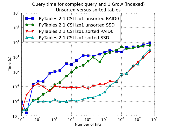
Figure 12. Times for complex queries with a cold cache (mean of 5 first random queries) for unsorted and sorted tables.

Even though we have shown many ways to improve query times that should fulfill the needs of most of people, for those needing more, you can for sure discover new optimization opportunities. For example, querying against sorted tables is limited mainly by sequential access to data on disk and data compression capability, so you may want to read Fine-tuning the chunksize, for ways on improving this aspect. Reading the other sections of this chapter will help in finding new roads for increasing the performance as well. You know, the limit for stopping the optimization process is basically your imagination (but, most plausibly, your available time ;-).

Compression issues

One of the beauties of PyTables is that it supports compression on tables and arrays [2], although it is not used by default. Compression of big amounts of data might be a bit controversial feature, because it has a legend of being a very big consumer of CPU time resources. However, if you are willing to check if compression can help not only by reducing your dataset file size but also by improving I/O efficiency, specially when dealing with very large datasets, keep reading.

A study on supported compression libraries

The compression library used by default is the Zlib (see [ZLIB]). Since HDF5 requires it, you can safely use it and expect that your HDF5 files will be readable on any other platform that has HDF5 libraries installed. Zlib provides good compression ratio, although somewhat slow, and reasonably fast decompression. Because of that, it is a good candidate to be used for compressing you data.

However, in some situations it is critical to have a very good decompression speed (at the expense of lower compression ratios or more CPU wasted on compression, as we will see soon). In others, the emphasis is put in achieving the maximum compression ratios, no matter which reading speed will result. This is why support for two additional compressors has been added to PyTables: LZO (see [LZO]) and bzip2 (see [BZIP2]). Following the author of LZO (and checked by the author of this section, as you will see soon), LZO offers pretty fast compression and extremely fast decompression. In fact, LZO is so fast when compressing/decompressing that it may well happen (that depends on your data, of course) that writing or reading a compressed dataset is sometimes faster than if it is not compressed at all (specially when dealing with extremely large datasets). This fact is very important, specially if you have to deal with very large amounts of data. Regarding bzip2, it has a reputation of achieving excellent compression ratios, but at the price of spending much more CPU time, which results in very low compression/decompression speeds.

Be aware that the LZO and bzip2 support in PyTables is not standard on HDF5, so if you are going to use your PyTables files in other contexts different from PyTables you will not be able to read them. Still, see the ptrepack (where the ptrepack utility is described) to find a way to free your files from LZO or bzip2 dependencies, so that you can use these compressors locally with the warranty that you can replace them with Zlib (or even remove compression completely) if you want to use these files with other HDF5 tools or platforms afterwards.

In order to allow you to grasp what amount of compression can be achieved, and how this affects performance, a series of experiments has been carried out. All the results presented in this section (and in the next one) have been obtained with synthetic data and using PyTables 1.3. Also, the tests have been conducted on a IBM OpenPower 720 (e-series) with a PowerPC G5 at 1.65 GHz and a hard disk spinning at 15K RPM. As your data and platform may be totally different for your case, take this just as a guide because your mileage may vary. Finally, and to be able to play with tables with a number of rows as large as possible, the record size has been chosen to be small (16 bytes). Here is its definition:

class Bench(IsDescription):
    var1 = StringCol(length=4)
    var2 = IntCol()
    var3 = FloatCol()

With this setup, you can look at the compression ratios that can be achieved in Figure 13. As you can see, LZO is the compressor that performs worse in this sense, but, curiously enough, there is not much difference between Zlib and bzip2.

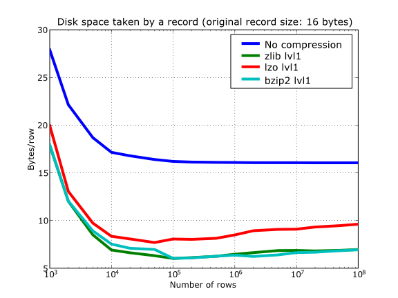
Figure 13. Comparison between different compression libraries.

Also, PyTables lets you select different compression levels for Zlib and bzip2, although you may get a bit disappointed by the small improvement that these compressors show when dealing with a combination of numbers and strings as in our example. As a reference, see plot Figure 14 for a comparison of the compression achieved by selecting different levels of Zlib. Very oddly, the best compression ratio corresponds to level 1 (!). See later for an explanation and more figures on this subject.

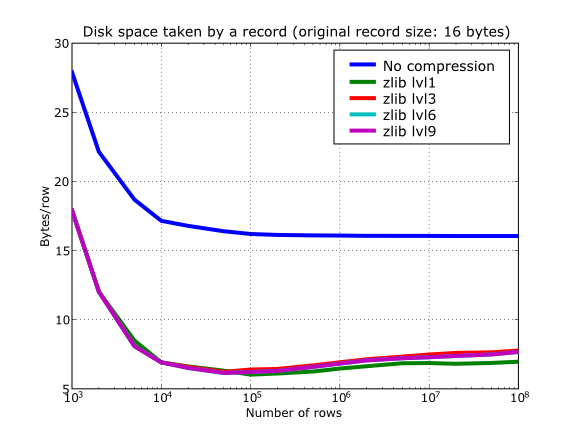
Figure 14. Comparison between different compression levels of Zlib.

Have also a look at Figure 15. It shows how the speed of writing rows evolves as the size (number of rows) of the table grows. Even though in these graphs the size of one single row is 16 bytes, you can most probably extrapolate these figures to other row sizes.

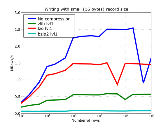
Figure 15. Writing tables with several compressors.

In Figure 16 you can see how compression affects the reading performance. In fact, what you see in the plot is an in-kernel selection speed, but provided that this operation is very fast (see In-kernel searches), we can accept it as an actual read test. Compared with the reference line without compression, the general trend here is that LZO does not affect too much the reading performance (and in some points it is actually better), Zlib makes speed drop to a half, while bzip2 is performing very slow (up to 8x slower).

Also, in the same Figure 16 you can notice some strange peaks in the speed that we might be tempted to attribute to libraries on which PyTables relies (HDF5, compressors...), or to PyTables itself. However, Figure 17 reveals that, if we put the file in the filesystem cache (by reading it several times before, for example), the evolution of the performance is much smoother. So, the most probable explanation would be that such peaks are a consequence of the underlying OS filesystem, rather than a flaw in PyTables (or any other library behind it). Another consequence that can be derived from the aforementioned plot is that LZO decompression performance is much better than Zlib, allowing an improvement in overall speed of more than 2x, and perhaps more important, the read performance for really large datasets (i.e. when they do not fit in the OS filesystem cache) can be actually better than not using compression at all. Finally, one can see that reading performance is very badly affected when bzip2 is used (it is 10x slower than LZO and 4x than Zlib), but this was somewhat expected anyway.

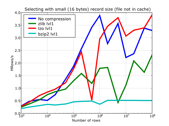
Figure 16. Selecting values in tables with several compressors. The file is not in the OS cache.

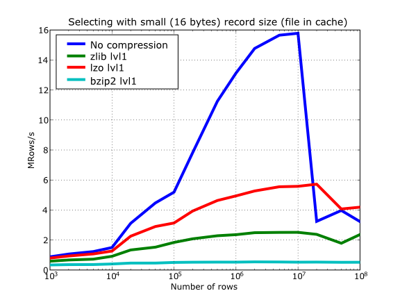
Figure 17. Selecting values in tables with several compressors. The file is in the OS cache.

So, generally speaking and looking at the experiments above, you can expect that LZO will be the fastest in both compressing and decompressing, but the one that achieves the worse compression ratio (although that may be just OK for many situations, specially when used with shuffling - see Shuffling (or how to make the compression process more effective)). bzip2 is the slowest, by large, in both compressing and decompressing, and besides, it does not achieve any better compression ratio than Zlib. Zlib represents a balance between them: it’s somewhat slow compressing (2x) and decompressing (3x) than LZO, but it normally achieves better compression ratios.

Finally, by looking at the plots Figure 18, Figure 19, and the aforementioned Figure 14 you can see why the recommended compression level to use for all compression libraries is 1. This is the lowest level of compression, but as the size of the underlying HDF5 chunk size is normally rather small compared with the size of compression buffers, there is not much point in increasing the latter (i.e. increasing the compression level). Nonetheless, in some situations (like for example, in extremely large tables or arrays, where the computed chunk size can be rather large) you may want to check, on your own, how the different compression levels do actually affect your application.

You can select the compression library and level by setting the complib and complevel keywords in the Filters class (see The Filters class). A compression level of 0 will completely disable compression (the default), 1 is the less memory and CPU time demanding level, while 9 is the maximum level and the most memory demanding and CPU intensive. Finally, have in mind that LZO is not accepting a compression level right now, so, when using LZO, 0 means that compression is not active, and any other value means that LZO is active.

So, in conclusion, if your ultimate goal is writing and reading as fast as possible, choose LZO. If you want to reduce as much as possible your data, while retaining acceptable read speed, choose Zlib. Finally, if portability is important for you, Zlib is your best bet. So, when you want to use bzip2? Well, looking at the results, it is difficult to recommend its use in general, but you may want to experiment with it in those cases where you know that it is well suited for your data pattern (for example, for dealing with repetitive string datasets).

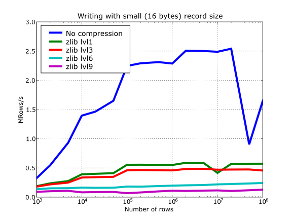
Figure 18. Writing in tables with different levels of compression.

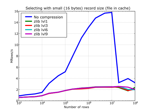
Figure 19. Selecting values in tables with different levels of compression. The file is in the OS cache.

Shuffling (or how to make the compression process more effective)

The HDF5 library provides an interesting filter that can leverage the results of your favorite compressor. Its name is shuffle, and because it can greatly benefit compression and it does not take many CPU resources (see below for a justification), it is active by default in PyTables whenever compression is activated (independently of the chosen compressor). It is deactivated when compression is off (which is the default, as you already should know). Of course, you can deactivate it if you want, but this is not recommended.

So, how does this mysterious filter exactly work? From the HDF5 reference manual:

"The shuffle filter de-interlaces a block of data by reordering the
bytes. All the bytes from one consistent byte position of each data
element are placed together in one block; all bytes from a second
consistent byte position of each data element are placed together a
second block; etc. For example, given three data elements of a 4-byte
datatype stored as 012301230123, shuffling will re-order data as
000111222333. This can be a valuable step in an effective compression
algorithm because the bytes in each byte position are often closely
related to each other and putting them together can increase the
compression ratio."

In Figure 20 you can see a benchmark that shows how the shuffle filter can help the different libraries in compressing data. In this experiment, shuffle has made LZO compress almost 3x more (!), while Zlib and bzip2 are seeing improvements of 2x. Once again, the data for this experiment is synthetic, and shuffle seems to do a great work with it, but in general, the results will vary in each case [3].

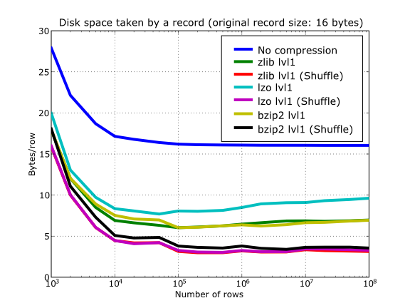
Figure 20. Comparison between different compression libraries with and without the shuffle filter.

At any rate, the most remarkable fact about the shuffle filter is the relatively high level of compression that compressor filters can achieve when used in combination with it. A curious thing to note is that the Bzip2 compression rate does not seem very much improved (less than a 40%), and what is more striking, Bzip2+shuffle does compress quite less than Zlib+shuffle or LZO+shuffle combinations, which is kind of unexpected. The thing that seems clear is that Bzip2 is not very good at compressing patterns that result of shuffle application. As always, you may want to experiment with your own data before widely applying the Bzip2+shuffle combination in order to avoid surprises.

Now, how does shuffling affect performance? Well, if you look at plots Figure 21, Figure 22 and Figure 23, you will get a somewhat unexpected (but pleasant) surprise. Roughly, shuffle makes the writing process (shuffling+compressing) faster (approximately a 15% for LZO, 30% for Bzip2 and a 80% for Zlib), which is an interesting result by itself. But perhaps more exciting is the fact that the reading process (unshuffling+decompressing) is also accelerated by a similar extent (a 20% for LZO, 60% for Zlib and a 75% for Bzip2, roughly).

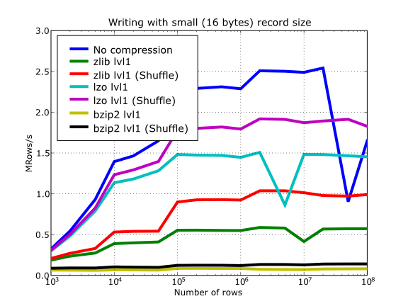
Figure 21. Writing with different compression libraries with and without the shuffle filter.

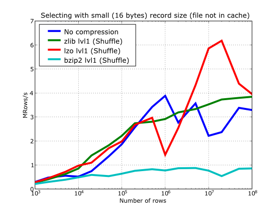
Figure 22. Reading with different compression libraries with the shuffle filter. The file is not in OS cache.

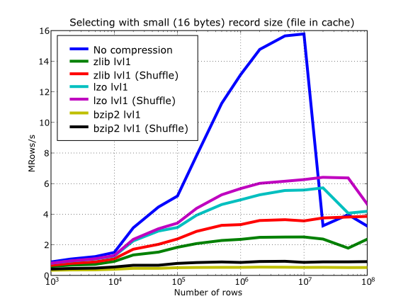
Figure 23. Reading with different compression libraries with and without the shuffle filter. The file is in OS cache.

You may wonder why introducing another filter in the write/read pipelines does effectively accelerate the throughput. Well, maybe data elements are more similar or related column-wise than row-wise, i.e. contiguous elements in the same column are more alike, so shuffling makes the job of the compressor easier (faster) and more effective (greater ratios). As a side effect, compressed chunks do fit better in the CPU cache (at least, the chunks are smaller!) so that the process of unshuffle/decompress can make a better use of the cache (i.e. reducing the number of CPU cache faults).

So, given the potential gains (faster writing and reading, but specially much improved compression level), it is a good thing to have such a filter enabled by default in the battle for discovering redundancy when you want to compress your data, just as PyTables does.

Using Psyco

Psyco (see [PSYCO]) is a kind of specialized compiler for Python that typically accelerates Python applications with no change in source code. You can think of Psyco as a kind of just-in-time (JIT) compiler, a little bit like Java’s, that emits machine code on the fly instead of interpreting your Python program step by step. The result is that your unmodified Python programs run faster.

Psyco is very easy to install and use, so in most scenarios it is worth to give it a try. However, it only runs on Intel 386 architectures, so if you are using other architectures, you are out of luck (and, moreover, it seems that there are no plans to support other platforms). Besides, with the addition of flexible (and very fast) in-kernel queries (by the way, they cannot be optimized at all by Psyco), the use of Psyco will only help in rather few scenarios. In fact, the only important situation that you might benefit right now from using Psyco (I mean, in PyTables contexts) is for speeding-up the write speed in tables when using the Row interface (see The Row class). But again, this latter case can also be accelerated by using the Table.append() method and building your own buffers [4].

As an example, imagine that you have a small script that reads and selects data over a series of datasets, like this:

def read_file(filename):
    "Select data from all the tables in filename"
    fileh = open_file(filename, mode = "r")
    result = []
    for table in fileh("/", 'Table'):
        result = [p['var3'] for p in table if p['var2'] <= 20]
    fileh.close()
    return result

if __name__=="__main__":
    print(read_file("myfile.h5"))

In order to accelerate this piece of code, you can rewrite your main program to look like:

if __name__=="__main__":
    import psyco
    psyco.bind(read_file)
    print(read_file("myfile.h5"))

That’s all! From now on, each time that you execute your Python script, Psyco will deploy its sophisticated algorithms so as to accelerate your calculations.

You can see in the graphs Figure 24 and Figure 25 how much I/O speed improvement you can get by using Psyco. By looking at this figures you can get an idea if these improvements are of your interest or not. In general, if you are not going to use compression you will take advantage of Psyco if your tables are medium sized (from a thousand to a million rows), and this advantage will disappear progressively when the number of rows grows well over one million. However if you use compression, you will probably see improvements even beyond this limit (see Compression issues). As always, there is no substitute for experimentation with your own dataset.

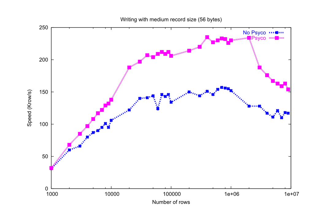
Figure 24. Writing tables with/without Psyco.

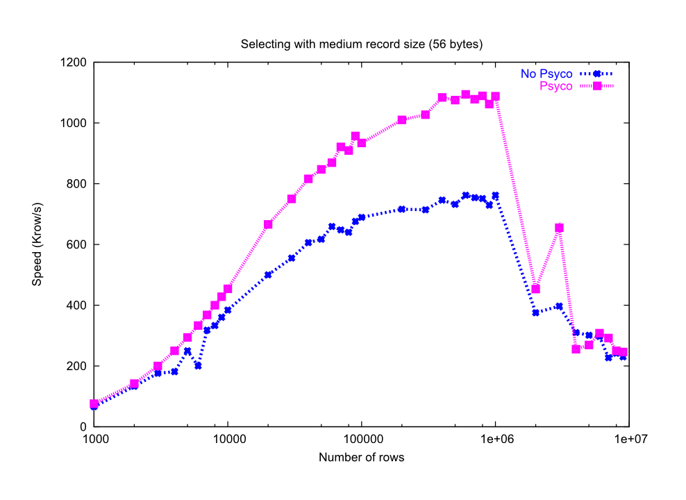
Figure 25. Reading tables with/without Psyco.

Getting the most from the node LRU cache

One limitation of the initial versions of PyTables was that they needed to load all nodes in a file completely before being ready to deal with them, making the opening times for files with a lot of nodes very high and unacceptable in many cases.

Starting from PyTables 1.2 on, a new lazy node loading schema was setup that avoids loading all the nodes of the object tree in memory. In addition, a new LRU cache was introduced in order to accelerate the access to already visited nodes. This cache (one per file) is responsible for keeping up the most recently visited nodes in memory and discard the least recent used ones. This represents a big advantage over the old schema, not only in terms of memory usage (as there is no need to load every node in memory), but it also adds very convenient optimizations for working interactively like, for example, speeding-up the opening times of files with lots of nodes, allowing to open almost any kind of file in typically less than one tenth of second (compare this with the more than 10 seconds for files with more than 10000 nodes in PyTables pre-1.2 era) as well as optimizing the access to frequently visited nodes. See for more info on the advantages (and also drawbacks) of this approach.

One thing that deserves some discussion is the election of the parameter that sets the maximum amount of nodes to be kept in memory at any time. As PyTables is meant to be deployed in machines that can have potentially low memory, the default for it is quite conservative (you can look at its actual value in the parameters.NODE_CACHE_SLOTS parameter in module tables/parameters.py). However, if you usually need to deal with files that have many more nodes than the maximum default, and you have a lot of free memory in your system, then you may want to experiment in order to see which is the appropriate value of parameters.NODE_CACHE_SLOTS that fits better your needs.

As an example, look at the next code:

def browse_tables(filename):
    fileh = open_file(filename,'a')
    group = fileh.root.newgroup
    for j in range(10):
        for tt in fileh.walk_nodes(group, "Table"):
            title = tt.attrs.TITLE
            for row in tt:
                pass
    fileh.close()

We will be running the code above against a couple of files having a /newgroup containing 100 tables and 1000 tables respectively. In addition, this benchmark is run twice for two different values of the LRU cache size, specifically 256 and 1024. You can see the results in table.

Retrieval speed and memory consumption depending on the number of nodes in LRU cache.

Number:		100 nodes				1000 nodes
Mem & Speed		Memory (MB)		Time (ms)		Memory (MB)		Time (ms)
Node is coming from...	Cache size	256	1024	256	1024	256	1024	256	1024
Disk		14	14	1.24	1.24	51	66	1.33	1.31
Cache		14	14	0.53	0.52	65	73	1.35	0.68

From the data in table, one can see that when the number of objects that you are dealing with does fit in cache, you will get better access times to them. Also, incrementing the node cache size effectively consumes more memory only if the total nodes exceeds the slots in cache; otherwise the memory consumption remains the same. It is also worth noting that incrementing the node cache size in the case you want to fit all your nodes in cache does not take much more memory than being too conservative. On the other hand, it might happen that the speed-up that you can achieve by allocating more slots in your cache is not worth the amount of memory used.

Also worth noting is that if you have a lot of memory available and performance is absolutely critical, you may want to try out a negative value for parameters.NODE_CACHE_SLOTS. This will cause that all the touched nodes will be kept in an internal dictionary and this is the faster way to load/retrieve nodes. However, and in order to avoid a large memory consumption, the user will be warned when the number of loaded nodes will reach the -NODE_CACHE_SLOTS value.

Finally, a value of zero in parameters.NODE_CACHE_SLOTS means that any cache mechanism is disabled.

At any rate, if you feel that this issue is important for you, there is no replacement for setting your own experiments up in order to proceed to fine-tune the parameters.NODE_CACHE_SLOTS parameter.

Note

PyTables >= 2.3 sports an optimized LRU cache node written in C, so you should expect significantly faster LRU cache operations when working with it.

Note

Numerical results reported in table have been obtained with PyTables < 3.1. In PyTables 3.1 the node cache mechanism has been completely redesigned so while all comments above are still valid, numerical values could be a little bit different from the ones reported in table.

Compacting your PyTables files

Let’s suppose that you have a file where you have made a lot of row deletions on one or more tables, or deleted many leaves or even entire subtrees. These operations might leave holes (i.e. space that is not used anymore) in your files that may potentially affect not only the size of the files but, more importantly, the performance of I/O. This is because when you delete a lot of rows in a table, the space is not automatically recovered on the fly. In addition, if you add many more rows to a table than specified in the expectedrows keyword at creation time this may affect performance as well, as explained in Informing PyTables about expected number of rows in tables or arrays.

In order to cope with these issues, you should be aware that PyTables includes a handy utility called ptrepack which can be very useful not only to compact fragmented files, but also to adjust some internal parameters in order to use better buffer and chunk sizes for optimum I/O speed. Please check the ptrepack for a brief tutorial on its use.

Another thing that you might want to use ptrepack for is changing the compression filters or compression levels on your existing data for different goals, like checking how this can affect both final size and I/O performance, or getting rid of the optional compressors like LZO or bzip2 in your existing files, in case you want to use them with generic HDF5 tools that do not have support for these filters.

---

[1]	CArray nodes, though not extensible, are chunked and have their optimum chunk size automatically computed at creation time, since their final shape is known.

[2]	Except for Array objects.

[3]	Some users reported that the typical improvement with real data is between a factor 1.5x and 2.5x over the already compressed datasets.

[4]	So, there is not much point in using Psyco with recent versions of PyTables anymore.