scipy.stats.tukeylambda

scipy.stats.tukeylambda = <scipy.stats._continuous_distns.tukeylambda_gen object at 0x596c610>

A Tukey-Lamdba continuous random variable.

As an instance of the rv_continuous class, tukeylambda object inherits from it a collection of generic methods (see below for the full list), and completes them with details specific for this particular distribution.

Notes

A flexible distribution, able to represent and interpolate between the following distributions:

• Cauchy (lam=-1)
• logistic (lam=0.0)
• approx Normal (lam=0.14)
• u-shape (lam = 0.5)
• uniform from -1 to 1 (lam = 1)

tukeylambda takes lam as a shape parameter.

The probability density above is defined in the “standardized” form. To shift and/or scale the distribution use the loc and scale parameters. Specifically, tukeylambda.pdf(x, lam, loc, scale) is identically equivalent to tukeylambda.pdf(y, lam) / scale with y = (x - loc) / scale.

Examples

>>> from scipy.stats import tukeylambda
>>> import matplotlib.pyplot as plt
>>> fig, ax = plt.subplots(1, 1)

Calculate a few first moments:

>>> lam = 3.13
>>> mean, var, skew, kurt = tukeylambda.stats(lam, moments='mvsk')

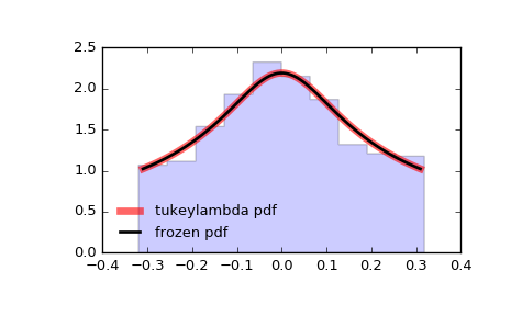
Display the probability density function (pdf):

>>> x = np.linspace(tukeylambda.ppf(0.01, lam),
...                 tukeylambda.ppf(0.99, lam), 100)
>>> ax.plot(x, tukeylambda.pdf(x, lam),
...        'r-', lw=5, alpha=0.6, label='tukeylambda pdf')

Alternatively, the distribution object can be called (as a function) to fix the shape, location and scale parameters. This returns a “frozen” RV object holding the given parameters fixed.

Freeze the distribution and display the frozen pdf:

>>> rv = tukeylambda(lam)
>>> ax.plot(x, rv.pdf(x), 'k-', lw=2, label='frozen pdf')

Check accuracy of cdf and ppf:

>>> vals = tukeylambda.ppf([0.001, 0.5, 0.999], lam)
>>> np.allclose([0.001, 0.5, 0.999], tukeylambda.cdf(vals, lam))
True

Generate random numbers:

>>> r = tukeylambda.rvs(lam, size=1000)

And compare the histogram:

>>> ax.hist(r, normed=True, histtype='stepfilled', alpha=0.2)
>>> ax.legend(loc='best', frameon=False)
>>> plt.show()

(Source code)

Methods

rvs(lam, loc=0, scale=1, size=1, random_state=None)	Random variates.
pdf(x, lam, loc=0, scale=1)	Probability density function.
logpdf(x, lam, loc=0, scale=1)	Log of the probability density function.
cdf(x, lam, loc=0, scale=1)	Cumulative density function.
logcdf(x, lam, loc=0, scale=1)	Log of the cumulative density function.
sf(x, lam, loc=0, scale=1)	Survival function (also defined as 1 - cdf, but sf is sometimes more accurate).
logsf(x, lam, loc=0, scale=1)	Log of the survival function.
ppf(q, lam, loc=0, scale=1)	Percent point function (inverse of cdf — percentiles).
isf(q, lam, loc=0, scale=1)	Inverse survival function (inverse of sf).
moment(n, lam, loc=0, scale=1)	Non-central moment of order n
stats(lam, loc=0, scale=1, moments='mv')	Mean(‘m’), variance(‘v’), skew(‘s’), and/or kurtosis(‘k’).
entropy(lam, loc=0, scale=1)	(Differential) entropy of the RV.
fit(data, lam, loc=0, scale=1)	Parameter estimates for generic data.
expect(func, args=(lam,), loc=0, scale=1, lb=None, ub=None, conditional=False, **kwds)	Expected value of a function (of one argument) with respect to the distribution.
median(lam, loc=0, scale=1)	Median of the distribution.
mean(lam, loc=0, scale=1)	Mean of the distribution.
var(lam, loc=0, scale=1)	Variance of the distribution.
std(lam, loc=0, scale=1)	Standard deviation of the distribution.
interval(alpha, lam, loc=0, scale=1)	Endpoints of the range that contains alpha percent of the distribution