
2.3. Clustering
Clustering of
unlabeled data can be performed with the module sklearn.cluster.
Each clustering algorithm comes in two variants: a class, that implements
the fit method to learn the clusters on train data, and a function,
that, given train data, returns an array of integer labels corresponding
to the different clusters. For the class, the labels over the training
data can be found in the labels_ attribute.
Input data
One important thing to note is that the algorithms implemented in
this module can take different kinds of matrix as input. All the
methods accept standard data matrices of shape [n_samples, n_features].
These can be obtained from the classes in the sklearn.feature_extraction
module. For AffinityPropagation, SpectralClustering
and DBSCAN one can also input similarity matrices of shape
[n_samples, n_samples]. These can be obtained from the functions
in the sklearn.metrics.pairwise module.
2.3.1. Overview of clustering methods
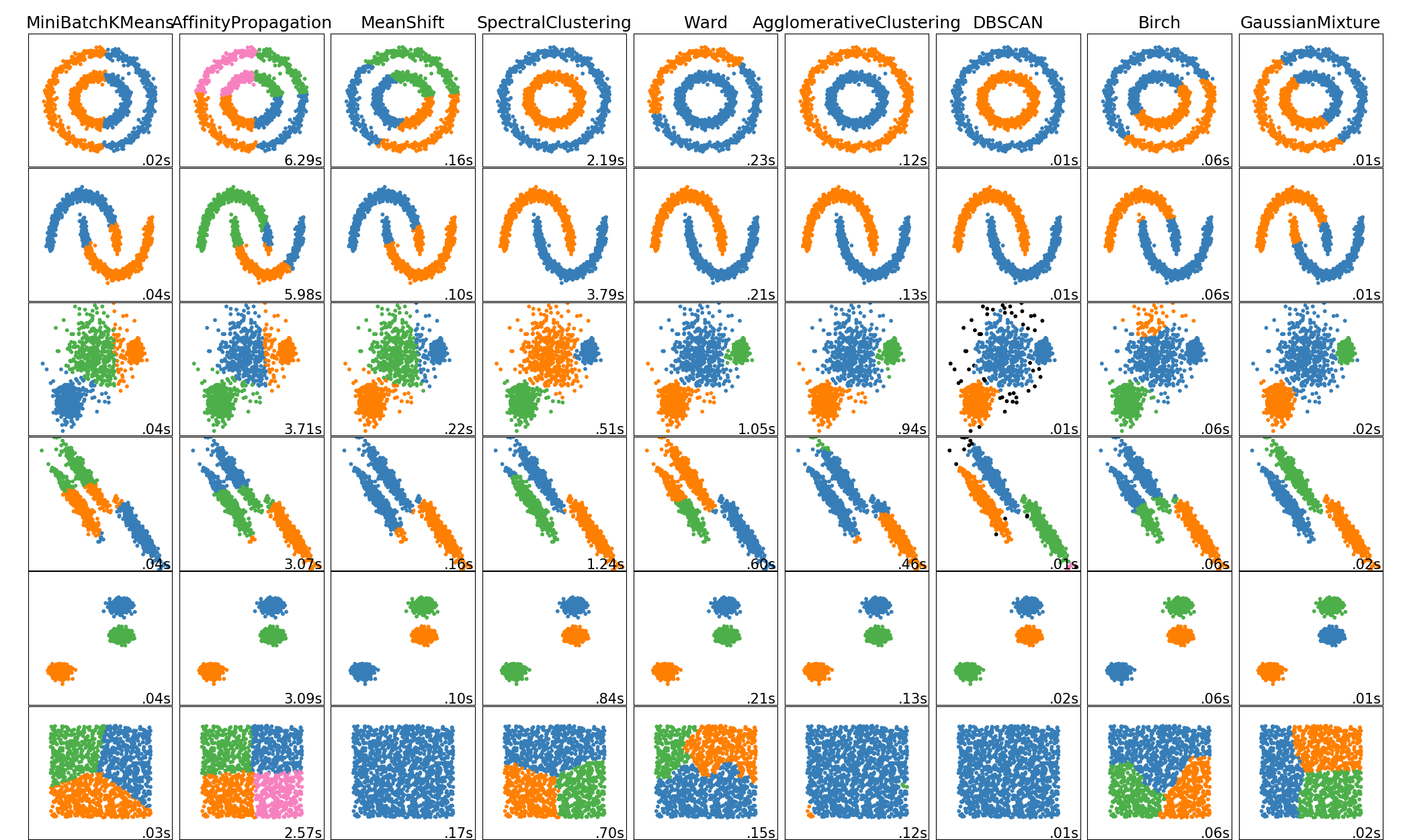
A comparison of the clustering algorithms in scikit-learn
| Method name | Parameters | Scalability | Usecase | Geometry (metric used) |
|---|---|---|---|---|
| K-Means | number of clusters | Very large n_samples, medium n_clusters with
MiniBatch code |
General-purpose, even cluster size, flat geometry, not too many clusters | Distances between points |
| Affinity propagation | damping, sample preference | Not scalable with n_samples | Many clusters, uneven cluster size, non-flat geometry | Graph distance (e.g. nearest-neighbor graph) |
| Mean-shift | bandwidth | Not scalable with n_samples |
Many clusters, uneven cluster size, non-flat geometry | Distances between points |
| Spectral clustering | number of clusters | Medium n_samples, small n_clusters |
Few clusters, even cluster size, non-flat geometry | Graph distance (e.g. nearest-neighbor graph) |
| Ward hierarchical clustering | number of clusters | Large n_samples and n_clusters |
Many clusters, possibly connectivity constraints | Distances between points |
| Agglomerative clustering | number of clusters, linkage type, distance | Large n_samples and n_clusters |
Many clusters, possibly connectivity constraints, non Euclidean distances | Any pairwise distance |
| DBSCAN | neighborhood size | Very large n_samples, medium n_clusters |
Non-flat geometry, uneven cluster sizes | Distances between nearest points |
| Gaussian mixtures | many | Not scalable | Flat geometry, good for density estimation | Mahalanobis distances to centers |
| Birch | branching factor, threshold, optional global clusterer. | Large n_clusters and n_samples |
Large dataset, outlier removal, data reduction. | Euclidean distance between points |
Non-flat geometry clustering is useful when the clusters have a specific shape, i.e. a non-flat manifold, and the standard euclidean distance is not the right metric. This case arises in the two top rows of the figure above.
Gaussian mixture models, useful for clustering, are described in another chapter of the documentation dedicated to mixture models. KMeans can be seen as a special case of Gaussian mixture model with equal covariance per component.
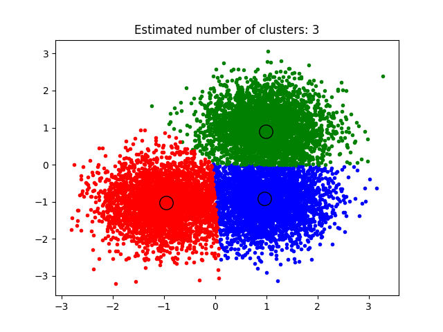
2.3.2. K-means
The KMeans algorithm clusters data by trying to separate samples
in n groups of equal variance, minimizing a criterion known as the
inertia or within-cluster sum-of-squares.
This algorithm requires the number of clusters to be specified.
It scales well to large number of samples and has been used
across a large range of application areas in many different fields.
The k-means algorithm divides a set of \(N\) samples \(X\) into \(K\) disjoint clusters \(C\), each described by the mean \(\mu_j\) of the samples in the cluster. The means are commonly called the cluster “centroids”; note that they are not, in general, points from \(X\), although they live in the same space. The K-means algorithm aims to choose centroids that minimise the inertia, or within-cluster sum of squared criterion:
Inertia, or the within-cluster sum of squares criterion, can be recognized as a measure of how internally coherent clusters are. It suffers from various drawbacks:
- Inertia makes the assumption that clusters are convex and isotropic, which is not always the case. It responds poorly to elongated clusters, or manifolds with irregular shapes.
- Inertia is not a normalized metric: we just know that lower values are better and zero is optimal. But in very high-dimensional spaces, Euclidean distances tend to become inflated (this is an instance of the so-called “curse of dimensionality”). Running a dimensionality reduction algorithm such as PCA prior to k-means clustering can alleviate this problem and speed up the computations.
K-means is often referred to as Lloyd’s algorithm. In basic terms, the algorithm has three steps. The first step chooses the initial centroids, with the most basic method being to choose \(k\) samples from the dataset \(X\). After initialization, K-means consists of looping between the two other steps. The first step assigns each sample to its nearest centroid. The second step creates new centroids by taking the mean value of all of the samples assigned to each previous centroid. The difference between the old and the new centroids are computed and the algorithm repeats these last two steps until this value is less than a threshold. In other words, it repeats until the centroids do not move significantly.
K-means is equivalent to the expectation-maximization algorithm with a small, all-equal, diagonal covariance matrix.
The algorithm can also be understood through the concept of Voronoi diagrams. First the Voronoi diagram of the points is calculated using the current centroids. Each segment in the Voronoi diagram becomes a separate cluster. Secondly, the centroids are updated to the mean of each segment. The algorithm then repeats this until a stopping criterion is fulfilled. Usually, the algorithm stops when the relative decrease in the objective function between iterations is less than the given tolerance value. This is not the case in this implementation: iteration stops when centroids move less than the tolerance.
Given enough time, K-means will always converge, however this may be to a local
minimum. This is highly dependent on the initialization of the centroids.
As a result, the computation is often done several times, with different
initializations of the centroids. One method to help address this issue is the
k-means++ initialization scheme, which has been implemented in scikit-learn
(use the init='k-means++' parameter). This initializes the centroids to be
(generally) distant from each other, leading to provably better results than
random initialization, as shown in the reference.
The algorithm supports sample weights, which can be given by a parameter
sample_weight. This allows to assign more weight to some samples when
computing cluster centers and values of inertia. For example, assigning a
weight of 2 to a sample is equivalent to adding a duplicate of that sample
to the dataset \(X\).
A parameter can be given to allow K-means to be run in parallel, called
n_jobs. Giving this parameter a positive value uses that many processors
(default: 1). A value of -1 uses all available processors, with -2 using one
less, and so on. Parallelization generally speeds up computation at the cost of
memory (in this case, multiple copies of centroids need to be stored, one for
each job).
Warning
The parallel version of K-Means is broken on OS X when numpy uses the Accelerate Framework. This is expected behavior: Accelerate can be called after a fork but you need to execv the subprocess with the Python binary (which multiprocessing does not do under posix).
K-means can be used for vector quantization. This is achieved using the
transform method of a trained model of KMeans.
Examples:
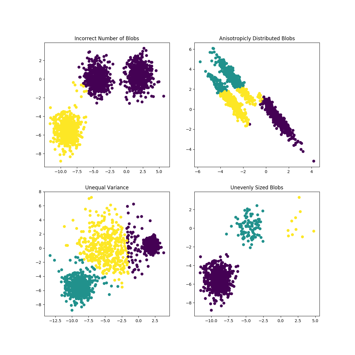
- Demonstration of k-means assumptions: Demonstrating when k-means performs intuitively and when it does not
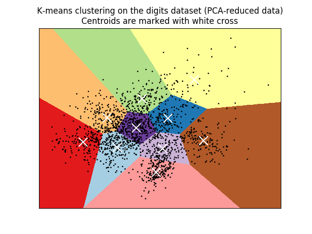
- A demo of K-Means clustering on the handwritten digits data: Clustering handwritten digits
References:
- “k-means++: The advantages of careful seeding” Arthur, David, and Sergei Vassilvitskii, Proceedings of the eighteenth annual ACM-SIAM symposium on Discrete algorithms, Society for Industrial and Applied Mathematics (2007)
2.3.2.1. Mini Batch K-Means
The MiniBatchKMeans is a variant of the KMeans algorithm
which uses mini-batches to reduce the computation time, while still attempting
to optimise the same objective function. Mini-batches are subsets of the input
data, randomly sampled in each training iteration. These mini-batches
drastically reduce the amount of computation required to converge to a local
solution. In contrast to other algorithms that reduce the convergence time of
k-means, mini-batch k-means produces results that are generally only slightly
worse than the standard algorithm.
The algorithm iterates between two major steps, similar to vanilla k-means. In the first step, \(b\) samples are drawn randomly from the dataset, to form a mini-batch. These are then assigned to the nearest centroid. In the second step, the centroids are updated. In contrast to k-means, this is done on a per-sample basis. For each sample in the mini-batch, the assigned centroid is updated by taking the streaming average of the sample and all previous samples assigned to that centroid. This has the effect of decreasing the rate of change for a centroid over time. These steps are performed until convergence or a predetermined number of iterations is reached.
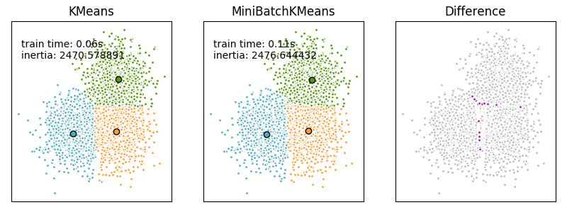
MiniBatchKMeans converges faster than KMeans, but the quality
of the results is reduced. In practice this difference in quality can be quite
small, as shown in the example and cited reference.
Examples:
- Comparison of the K-Means and MiniBatchKMeans clustering algorithms: Comparison of KMeans and MiniBatchKMeans
- Clustering text documents using k-means: Document clustering using sparse MiniBatchKMeans
- Online learning of a dictionary of parts of faces
References:
- “Web Scale K-Means clustering” D. Sculley, Proceedings of the 19th international conference on World wide web (2010)
2.3.3. Affinity Propagation
AffinityPropagation creates clusters by sending messages between
pairs of samples until convergence. A dataset is then described using a small
number of exemplars, which are identified as those most representative of other
samples. The messages sent between pairs represent the suitability for one
sample to be the exemplar of the other, which is updated in response to the
values from other pairs. This updating happens iteratively until convergence,
at which point the final exemplars are chosen, and hence the final clustering
is given.
Affinity Propagation can be interesting as it chooses the number of clusters based on the data provided. For this purpose, the two important parameters are the preference, which controls how many exemplars are used, and the damping factor which damps the responsibility and availability messages to avoid numerical oscillations when updating these messages.
The main drawback of Affinity Propagation is its complexity. The algorithm has a time complexity of the order \(O(N^2 T)\), where \(N\) is the number of samples and \(T\) is the number of iterations until convergence. Further, the memory complexity is of the order \(O(N^2)\) if a dense similarity matrix is used, but reducible if a sparse similarity matrix is used. This makes Affinity Propagation most appropriate for small to medium sized datasets.
Examples:
- Demo of affinity propagation clustering algorithm: Affinity Propagation on a synthetic 2D datasets with 3 classes.
- Visualizing the stock market structure Affinity Propagation on Financial time series to find groups of companies
Algorithm description: The messages sent between points belong to one of two categories. The first is the responsibility \(r(i, k)\), which is the accumulated evidence that sample \(k\) should be the exemplar for sample \(i\). The second is the availability \(a(i, k)\) which is the accumulated evidence that sample \(i\) should choose sample \(k\) to be its exemplar, and considers the values for all other samples that \(k\) should be an exemplar. In this way, exemplars are chosen by samples if they are (1) similar enough to many samples and (2) chosen by many samples to be representative of themselves.
More formally, the responsibility of a sample \(k\) to be the exemplar of sample \(i\) is given by:
Where \(s(i, k)\) is the similarity between samples \(i\) and \(k\). The availability of sample \(k\) to be the exemplar of sample \(i\) is given by:
To begin with, all values for \(r\) and \(a\) are set to zero, and the calculation of each iterates until convergence. As discussed above, in order to avoid numerical oscillations when updating the messages, the damping factor \(\lambda\) is introduced to iteration process:
where \(t\) indicates the iteration times.
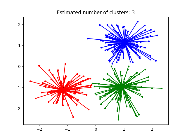
2.3.4. Mean Shift
MeanShift clustering aims to discover blobs in a smooth density of
samples. It is a centroid based algorithm, which works by updating candidates
for centroids to be the mean of the points within a given region. These
candidates are then filtered in a post-processing stage to eliminate
near-duplicates to form the final set of centroids.
Given a candidate centroid \(x_i\) for iteration \(t\), the candidate is updated according to the following equation:
Where \(N(x_i)\) is the neighborhood of samples within a given distance around \(x_i\) and \(m\) is the mean shift vector that is computed for each centroid that points towards a region of the maximum increase in the density of points. This is computed using the following equation, effectively updating a centroid to be the mean of the samples within its neighborhood:
The algorithm automatically sets the number of clusters, instead of relying on a
parameter bandwidth, which dictates the size of the region to search through.
This parameter can be set manually, but can be estimated using the provided
estimate_bandwidth function, which is called if the bandwidth is not set.
The algorithm is not highly scalable, as it requires multiple nearest neighbor searches during the execution of the algorithm. The algorithm is guaranteed to converge, however the algorithm will stop iterating when the change in centroids is small.
Labelling a new sample is performed by finding the nearest centroid for a given sample.
Examples:
- A demo of the mean-shift clustering algorithm: Mean Shift clustering on a synthetic 2D datasets with 3 classes.
References:
- “Mean shift: A robust approach toward feature space analysis.” D. Comaniciu and P. Meer, IEEE Transactions on Pattern Analysis and Machine Intelligence (2002)
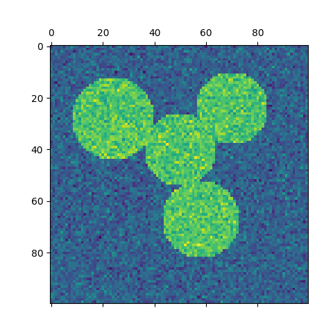
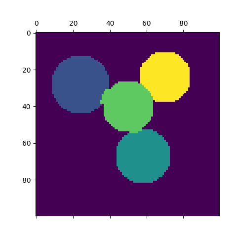
2.3.5. Spectral clustering
SpectralClustering does a low-dimension embedding of the
affinity matrix between samples, followed by a KMeans in the low
dimensional space. It is especially efficient if the affinity matrix is
sparse and the pyamg module is installed.
SpectralClustering requires the number of clusters to be specified. It
works well for a small number of clusters but is not advised when using
many clusters.
For two clusters, it solves a convex relaxation of the normalised cuts problem on the similarity graph: cutting the graph in two so that the weight of the edges cut is small compared to the weights of the edges inside each cluster. This criteria is especially interesting when working on images: graph vertices are pixels, and edges of the similarity graph are a function of the gradient of the image.
Warning
Transforming distance to well-behaved similarities
Note that if the values of your similarity matrix are not well distributed, e.g. with negative values or with a distance matrix rather than a similarity, the spectral problem will be singular and the problem not solvable. In which case it is advised to apply a transformation to the entries of the matrix. For instance, in the case of a signed distance matrix, is common to apply a heat kernel:
similarity = np.exp(-beta * distance / distance.std())
See the examples for such an application.
Examples:
- Spectral clustering for image segmentation: Segmenting objects from a noisy background using spectral clustering.
- Segmenting the picture of greek coins in regions: Spectral clustering to split the image of coins in regions.
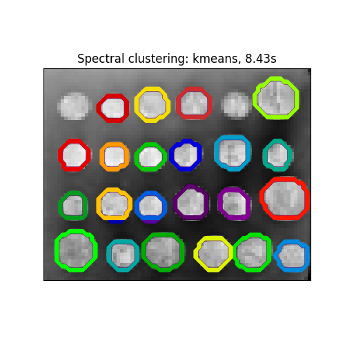
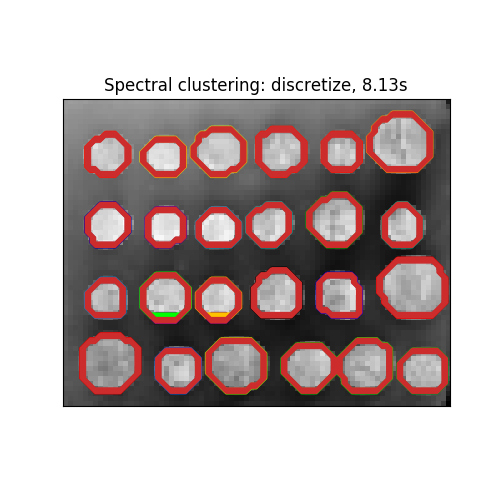
2.3.5.1. Different label assignment strategies
Different label assignment strategies can be used, corresponding to the
assign_labels parameter of SpectralClustering.
The "kmeans" strategy can match finer details of the data, but it can be
more unstable. In particular, unless you control the random_state, it
may not be reproducible from run-to-run, as it depends on a random
initialization. On the other hand, the "discretize" strategy is 100%
reproducible, but it tends to create parcels of fairly even and
geometrical shape.
assign_labels="kmeans" |
assign_labels="discretize" |
|---|---|
 |
 |
2.3.5.2. Spectral Clustering Graphs
Spectral Clustering can also be used to cluster graphs by their spectral embeddings. In this case, the affinity matrix is the adjacency matrix of the graph, and SpectralClustering is initialized with affinity=’precomputed’:
>>> from sklearn.cluster import SpectralClustering
>>> sc = SpectralClustering(3, affinity='precomputed', n_init=100,
...                         assign_labels='discretize')
>>> sc.fit_predict(adjacency_matrix)
References:
- “A Tutorial on Spectral Clustering” Ulrike von Luxburg, 2007
- “Normalized cuts and image segmentation” Jianbo Shi, Jitendra Malik, 2000
- “A Random Walks View of Spectral Segmentation” Marina Meila, Jianbo Shi, 2001
- “On Spectral Clustering: Analysis and an algorithm” Andrew Y. Ng, Michael I. Jordan, Yair Weiss, 2001
2.3.6. Hierarchical clustering
Hierarchical clustering is a general family of clustering algorithms that build nested clusters by merging or splitting them successively. This hierarchy of clusters is represented as a tree (or dendrogram). The root of the tree is the unique cluster that gathers all the samples, the leaves being the clusters with only one sample. See the Wikipedia page for more details.
The AgglomerativeClustering object performs a hierarchical clustering
using a bottom up approach: each observation starts in its own cluster, and
clusters are successively merged together. The linkage criteria determines the
metric used for the merge strategy:
- Ward minimizes the sum of squared differences within all clusters. It is a variance-minimizing approach and in this sense is similar to the k-means objective function but tackled with an agglomerative hierarchical approach.
- Maximum or complete linkage minimizes the maximum distance between observations of pairs of clusters.
- Average linkage minimizes the average of the distances between all observations of pairs of clusters.
- Single linkage minimizes the distance between the closest observations of pairs of clusters.
AgglomerativeClustering can also scale to large number of samples
when it is used jointly with a connectivity matrix, but is computationally
expensive when no connectivity constraints are added between samples: it
considers at each step all the possible merges.
The FeatureAgglomeration uses agglomerative clustering to
group together features that look very similar, thus decreasing the
number of features. It is a dimensionality reduction tool, see
Unsupervised dimensionality reduction.
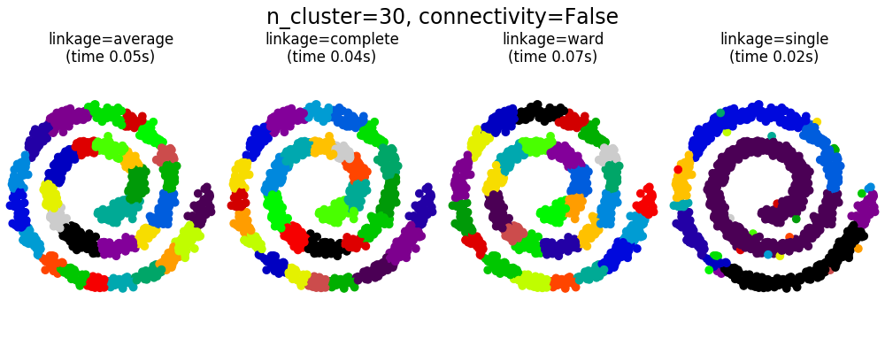
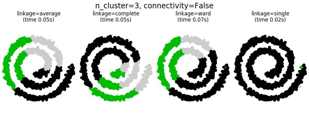
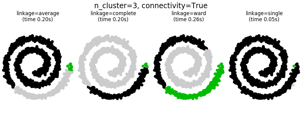
2.3.6.1. Different linkage type: Ward, complete, average, and single linkage
AgglomerativeClustering supports Ward, single, average, and complete
linkage strategies.
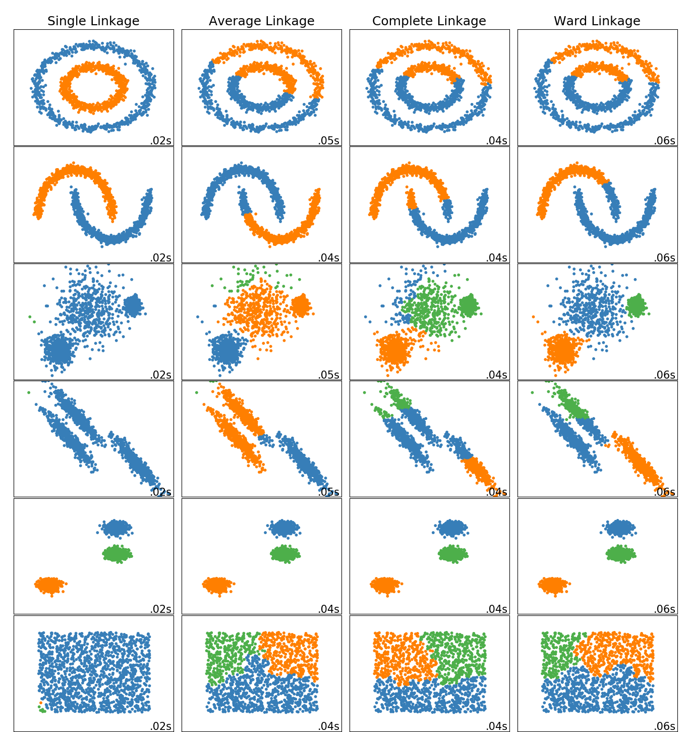
Agglomerative cluster has a “rich get richer” behavior that leads to uneven cluster sizes. In this regard, single linkage is the worst strategy, and Ward gives the most regular sizes. However, the affinity (or distance used in clustering) cannot be varied with Ward, thus for non Euclidean metrics, average linkage is a good alternative. Single linkage, while not robust to noisy data, can be computed very efficiently and can therefore be useful to provide hierarchical clustering of larger datasets. Single linkage can also perform well on non-globular data.
Examples:
- Various Agglomerative Clustering on a 2D embedding of digits: exploration of the different linkage strategies in a real dataset.
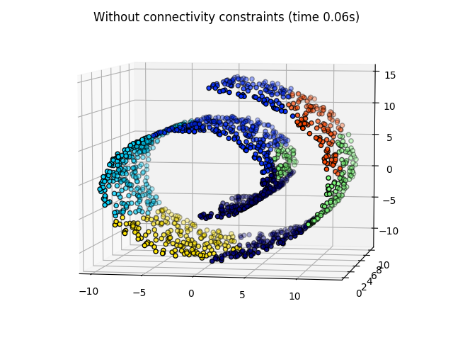
2.3.6.2. Adding connectivity constraints
An interesting aspect of AgglomerativeClustering is that
connectivity constraints can be added to this algorithm (only adjacent
clusters can be merged together), through a connectivity matrix that defines
for each sample the neighboring samples following a given structure of the
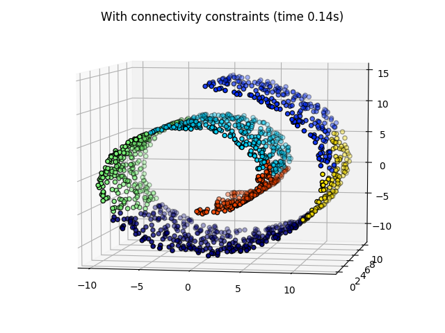
data. For instance, in the swiss-roll example below, the connectivity
constraints forbid the merging of points that are not adjacent on the swiss
roll, and thus avoid forming clusters that extend across overlapping folds of
the roll.
These constraint are useful to impose a certain local structure, but they also make the algorithm faster, especially when the number of the samples is high.
The connectivity constraints are imposed via an connectivity matrix: a
scipy sparse matrix that has elements only at the intersection of a row
and a column with indices of the dataset that should be connected. This
matrix can be constructed from a-priori information: for instance, you
may wish to cluster web pages by only merging pages with a link pointing
from one to another. It can also be learned from the data, for instance
using sklearn.neighbors.kneighbors_graph to restrict
merging to nearest neighbors as in this example, or
using sklearn.feature_extraction.image.grid_to_graph to
enable only merging of neighboring pixels on an image, as in the
coin example.
Examples:
- A demo of structured Ward hierarchical clustering on an image of coins: Ward clustering to split the image of coins in regions.
- Hierarchical clustering: structured vs unstructured ward: Example of Ward algorithm on a swiss-roll, comparison of structured approaches versus unstructured approaches.
- Feature agglomeration vs. univariate selection: Example of dimensionality reduction with feature agglomeration based on Ward hierarchical clustering.
- Agglomerative clustering with and without structure
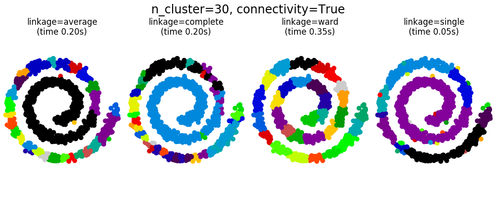
Warning
Connectivity constraints with single, average and complete linkage
Connectivity constraints and single, complete or average linkage can enhance
the ‘rich getting richer’ aspect of agglomerative clustering,
particularly so if they are built with
sklearn.neighbors.kneighbors_graph. In the limit of a small
number of clusters, they tend to give a few macroscopically occupied
clusters and almost empty ones. (see the discussion in
Agglomerative clustering with and without structure).
Single linkage is the most brittle linkage option with regard to this issue.
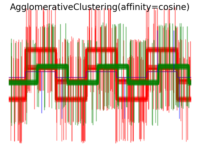
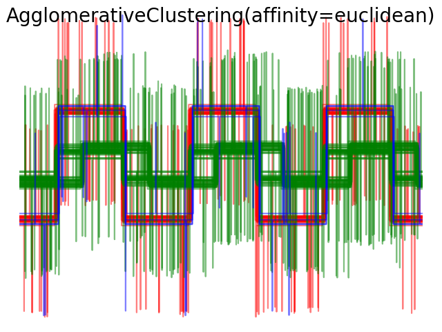
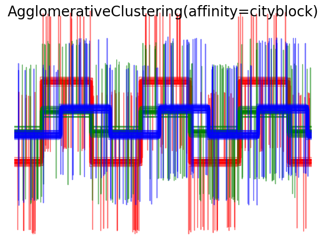
2.3.6.3. Varying the metric
Single, average and complete linkage can be used with a variety of distances (or affinities), in particular Euclidean distance (l2), Manhattan distance (or Cityblock, or l1), cosine distance, or any precomputed affinity matrix.
- l1 distance is often good for sparse features, or sparse noise: i.e. many of the features are zero, as in text mining using occurrences of rare words.
- cosine distance is interesting because it is invariant to global scalings of the signal.
The guidelines for choosing a metric is to use one that maximizes the distance between samples in different classes, and minimizes that within each class.
2.3.7. DBSCAN
The DBSCAN algorithm views clusters as areas of high density
separated by areas of low density. Due to this rather generic view, clusters
found by DBSCAN can be any shape, as opposed to k-means which assumes that
clusters are convex shaped. The central component to the DBSCAN is the concept
of core samples, which are samples that are in areas of high density. A
cluster is therefore a set of core samples, each close to each other
(measured by some distance measure)
and a set of non-core samples that are close to a core sample (but are not
themselves core samples). There are two parameters to the algorithm,
min_samples and eps,
which define formally what we mean when we say dense.
Higher min_samples or lower eps
indicate higher density necessary to form a cluster.
More formally, we define a core sample as being a sample in the dataset such
that there exist min_samples other samples within a distance of
eps, which are defined as neighbors of the core sample. This tells
us that the core sample is in a dense area of the vector space. A cluster
is a set of core samples that can be built by recursively taking a core
sample, finding all of its neighbors that are core samples, finding all of
their neighbors that are core samples, and so on. A cluster also has a
set of non-core samples, which are samples that are neighbors of a core sample
in the cluster but are not themselves core samples. Intuitively, these samples
are on the fringes of a cluster.
Any core sample is part of a cluster, by definition. Any sample that is not a
core sample, and is at least eps in distance from any core sample, is
considered an outlier by the algorithm.
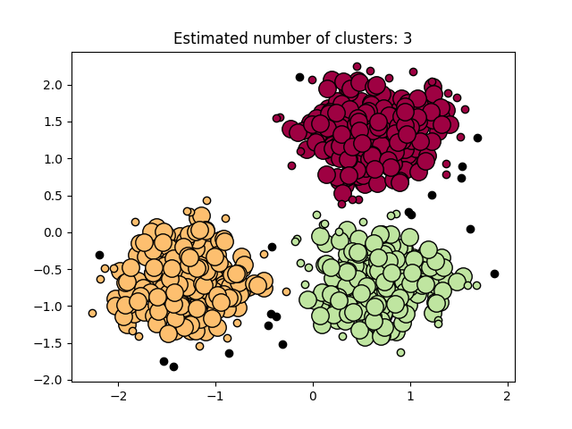
In the figure below, the color indicates cluster membership, with large circles indicating core samples found by the algorithm. Smaller circles are non-core samples that are still part of a cluster. Moreover, the outliers are indicated by black points below.
Examples:
Implementation
The DBSCAN algorithm is deterministic, always generating the same clusters
when given the same data in the same order. However, the results can differ when
data is provided in a different order. First, even though the core samples
will always be assigned to the same clusters, the labels of those clusters
will depend on the order in which those samples are encountered in the data.
Second and more importantly, the clusters to which non-core samples are assigned
can differ depending on the data order. This would happen when a non-core sample
has a distance lower than eps to two core samples in different clusters. By the
triangular inequality, those two core samples must be more distant than
eps from each other, or they would be in the same cluster. The non-core
sample is assigned to whichever cluster is generated first in a pass
through the data, and so the results will depend on the data ordering.
The current implementation uses ball trees and kd-trees
to determine the neighborhood of points,
which avoids calculating the full distance matrix
(as was done in scikit-learn versions before 0.14).
The possibility to use custom metrics is retained;
for details, see NearestNeighbors.
Memory consumption for large sample sizes
This implementation is by default not memory efficient because it constructs a full pairwise similarity matrix in the case where kd-trees or ball-trees cannot be used (e.g. with sparse matrices). This matrix will consume n^2 floats. A couple of mechanisms for getting around this are:
- A sparse radius neighborhood graph (where missing entries are presumed to
be out of eps) can be precomputed in a memory-efficient way and dbscan
can be run over this with
metric='precomputed'. Seesklearn.neighbors.NearestNeighbors.radius_neighbors_graph. - The dataset can be compressed, either by removing exact duplicates if
these occur in your data, or by using BIRCH. Then you only have a
relatively small number of representatives for a large number of points.
You can then provide a
sample_weightwhen fitting DBSCAN.
References:
- “A Density-Based Algorithm for Discovering Clusters in Large Spatial Databases with Noise” Ester, M., H. P. Kriegel, J. Sander, and X. Xu, In Proceedings of the 2nd International Conference on Knowledge Discovery and Data Mining, Portland, OR, AAAI Press, pp. 226–231. 1996
2.3.8. Birch
The Birch builds a tree called the Characteristic Feature Tree (CFT)
for the given data. The data is essentially lossy compressed to a set of
Characteristic Feature nodes (CF Nodes). The CF Nodes have a number of
subclusters called Characteristic Feature subclusters (CF Subclusters)
and these CF Subclusters located in the non-terminal CF Nodes
can have CF Nodes as children.
The CF Subclusters hold the necessary information for clustering which prevents the need to hold the entire input data in memory. This information includes:
- Number of samples in a subcluster.
- Linear Sum - A n-dimensional vector holding the sum of all samples
- Squared Sum - Sum of the squared L2 norm of all samples.
- Centroids - To avoid recalculation linear sum / n_samples.
- Squared norm of the centroids.
The Birch algorithm has two parameters, the threshold and the branching factor. The branching factor limits the number of subclusters in a node and the threshold limits the distance between the entering sample and the existing subclusters.
This algorithm can be viewed as an instance or data reduction method,
since it reduces the input data to a set of subclusters which are obtained directly
from the leaves of the CFT. This reduced data can be further processed by feeding
it into a global clusterer. This global clusterer can be set by n_clusters.
If n_clusters is set to None, the subclusters from the leaves are directly
read off, otherwise a global clustering step labels these subclusters into global
clusters (labels) and the samples are mapped to the global label of the nearest subcluster.
Algorithm description:
- A new sample is inserted into the root of the CF Tree which is a CF Node. It is then merged with the subcluster of the root, that has the smallest radius after merging, constrained by the threshold and branching factor conditions. If the subcluster has any child node, then this is done repeatedly till it reaches a leaf. After finding the nearest subcluster in the leaf, the properties of this subcluster and the parent subclusters are recursively updated.
- If the radius of the subcluster obtained by merging the new sample and the nearest subcluster is greater than the square of the threshold and if the number of subclusters is greater than the branching factor, then a space is temporarily allocated to this new sample. The two farthest subclusters are taken and the subclusters are divided into two groups on the basis of the distance between these subclusters.
- If this split node has a parent subcluster and there is room for a new subcluster, then the parent is split into two. If there is no room, then this node is again split into two and the process is continued recursively, till it reaches the root.
Birch or MiniBatchKMeans?
- Birch does not scale very well to high dimensional data. As a rule of thumb if
n_featuresis greater than twenty, it is generally better to use MiniBatchKMeans.- If the number of instances of data needs to be reduced, or if one wants a large number of subclusters either as a preprocessing step or otherwise, Birch is more useful than MiniBatchKMeans.
How to use partial_fit?
To avoid the computation of global clustering, for every call of partial_fit
the user is advised
- To set
n_clusters=Noneinitially- Train all data by multiple calls to partial_fit.
- Set
n_clustersto a required value usingbrc.set_params(n_clusters=n_clusters).- Call
partial_fitfinally with no arguments, i.e.brc.partial_fit()which performs the global clustering.

References:
- Tian Zhang, Raghu Ramakrishnan, Maron Livny BIRCH: An efficient data clustering method for large databases. http://www.cs.sfu.ca/CourseCentral/459/han/papers/zhang96.pdf
- Roberto Perdisci JBirch - Java implementation of BIRCH clustering algorithm https://code.google.com/archive/p/jbirch
2.3.9. Clustering performance evaluation
Evaluating the performance of a clustering algorithm is not as trivial as counting the number of errors or the precision and recall of a supervised classification algorithm. In particular any evaluation metric should not take the absolute values of the cluster labels into account but rather if this clustering define separations of the data similar to some ground truth set of classes or satisfying some assumption such that members belong to the same class are more similar that members of different classes according to some similarity metric.
2.3.9.1. Adjusted Rand index
Given the knowledge of the ground truth class assignments labels_true
and our clustering algorithm assignments of the same samples
labels_pred, the adjusted Rand index is a function that measures
the similarity of the two assignments, ignoring permutations and with
chance normalization:
>>> from sklearn import metrics
>>> labels_true = [0, 0, 0, 1, 1, 1]
>>> labels_pred = [0, 0, 1, 1, 2, 2]

>>> metrics.adjusted_rand_score(labels_true, labels_pred)
0.24...
One can permute 0 and 1 in the predicted labels, rename 2 to 3, and get the same score:
>>> labels_pred = [1, 1, 0, 0, 3, 3]
>>> metrics.adjusted_rand_score(labels_true, labels_pred)
0.24...
Furthermore, adjusted_rand_score is symmetric: swapping the argument
does not change the score. It can thus be used as a consensus
measure:
>>> metrics.adjusted_rand_score(labels_pred, labels_true)
0.24...
Perfect labeling is scored 1.0:
>>> labels_pred = labels_true[:]
>>> metrics.adjusted_rand_score(labels_true, labels_pred)
1.0
Bad (e.g. independent labelings) have negative or close to 0.0 scores:
>>> labels_true = [0, 1, 2, 0, 3, 4, 5, 1]
>>> labels_pred = [1, 1, 0, 0, 2, 2, 2, 2]
>>> metrics.adjusted_rand_score(labels_true, labels_pred)
-0.12...
2.3.9.1.1. Advantages
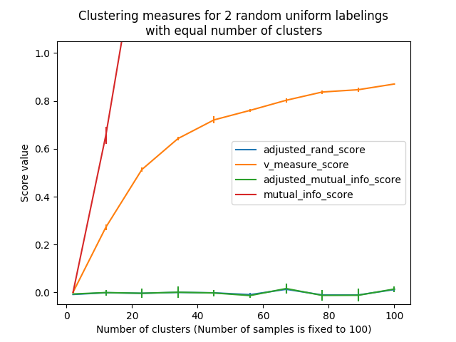
- Random (uniform) label assignments have a ARI score close to 0.0
for any value of
n_clustersandn_samples(which is not the case for raw Rand index or the V-measure for instance). - Bounded range [-1, 1]: negative values are bad (independent labelings), similar clusterings have a positive ARI, 1.0 is the perfect match score.
- No assumption is made on the cluster structure: can be used to compare clustering algorithms such as k-means which assumes isotropic blob shapes with results of spectral clustering algorithms which can find cluster with “folded” shapes.
2.3.9.1.2. Drawbacks
Contrary to inertia, ARI requires knowledge of the ground truth classes while is almost never available in practice or requires manual assignment by human annotators (as in the supervised learning setting).
However ARI can also be useful in a purely unsupervised setting as a building block for a Consensus Index that can be used for clustering model selection (TODO).
Examples:
- Adjustment for chance in clustering performance evaluation: Analysis of the impact of the dataset size on the value of clustering measures for random assignments.
2.3.9.1.3. Mathematical formulation
If C is a ground truth class assignment and K the clustering, let us define \(a\) and \(b\) as:
- \(a\), the number of pairs of elements that are in the same set in C and in the same set in K
- \(b\), the number of pairs of elements that are in different sets in C and in different sets in K
The raw (unadjusted) Rand index is then given by:
Where \(C_2^{n_{samples}}\) is the total number of possible pairs in the dataset (without ordering).
However the RI score does not guarantee that random label assignments will get a value close to zero (esp. if the number of clusters is in the same order of magnitude as the number of samples).
To counter this effect we can discount the expected RI \(E[\text{RI}]\) of random labelings by defining the adjusted Rand index as follows:
References
- Comparing Partitions L. Hubert and P. Arabie, Journal of Classification 1985
- Wikipedia entry for the adjusted Rand index
2.3.9.2. Mutual Information based scores
Given the knowledge of the ground truth class assignments labels_true and
our clustering algorithm assignments of the same samples labels_pred, the
Mutual Information is a function that measures the agreement of the two
assignments, ignoring permutations. Two different normalized versions of this
measure are available, Normalized Mutual Information (NMI) and Adjusted
Mutual Information (AMI). NMI is often used in the literature, while AMI was
proposed more recently and is normalized against chance:
>>> from sklearn import metrics
>>> labels_true = [0, 0, 0, 1, 1, 1]
>>> labels_pred = [0, 0, 1, 1, 2, 2]

>>> metrics.adjusted_mutual_info_score(labels_true, labels_pred)
0.22504...
One can permute 0 and 1 in the predicted labels, rename 2 to 3 and get the same score:
>>> labels_pred = [1, 1, 0, 0, 3, 3]
>>> metrics.adjusted_mutual_info_score(labels_true, labels_pred)
0.22504...
All, mutual_info_score, adjusted_mutual_info_score and
normalized_mutual_info_score are symmetric: swapping the argument does
not change the score. Thus they can be used as a consensus measure:
>>> metrics.adjusted_mutual_info_score(labels_pred, labels_true)
0.22504...
Perfect labeling is scored 1.0:
>>> labels_pred = labels_true[:]
>>> metrics.adjusted_mutual_info_score(labels_true, labels_pred)
1.0

>>> metrics.normalized_mutual_info_score(labels_true, labels_pred)
1.0
This is not true for mutual_info_score, which is therefore harder to judge:
>>> metrics.mutual_info_score(labels_true, labels_pred)
0.69...
Bad (e.g. independent labelings) have non-positive scores:
>>> labels_true = [0, 1, 2, 0, 3, 4, 5, 1]
>>> labels_pred = [1, 1, 0, 0, 2, 2, 2, 2]
>>> metrics.adjusted_mutual_info_score(labels_true, labels_pred)
-0.10526...
2.3.9.2.1. Advantages
- Random (uniform) label assignments have a AMI score close to 0.0
for any value of
n_clustersandn_samples(which is not the case for raw Mutual Information or the V-measure for instance). - Upper bound of 1: Values close to zero indicate two label assignments that are largely independent, while values close to one indicate significant agreement. Further, an AMI of exactly 1 indicates that the two label assignments are equal (with or without permutation).
2.3.9.2.2. Drawbacks
Contrary to inertia, MI-based measures require the knowledge of the ground truth classes while almost never available in practice or requires manual assignment by human annotators (as in the supervised learning setting).
However MI-based measures can also be useful in purely unsupervised setting as a building block for a Consensus Index that can be used for clustering model selection.
NMI and MI are not adjusted against chance.
Examples:
- Adjustment for chance in clustering performance evaluation: Analysis of the impact of the dataset size on the value of clustering measures for random assignments. This example also includes the Adjusted Rand Index.
2.3.9.2.3. Mathematical formulation
Assume two label assignments (of the same N objects), \(U\) and \(V\). Their entropy is the amount of uncertainty for a partition set, defined by:
where \(P(i) = |U_i| / N\) is the probability that an object picked at random from \(U\) falls into class \(U_i\). Likewise for \(V\):
With \(P'(j) = |V_j| / N\). The mutual information (MI) between \(U\) and \(V\) is calculated by:
where \(P(i, j) = |U_i \cap V_j| / N\) is the probability that an object picked at random falls into both classes \(U_i\) and \(V_j\).
It also can be expressed in set cardinality formulation:
The normalized mutual information is defined as
This value of the mutual information and also the normalized variant is not adjusted for chance and will tend to increase as the number of different labels (clusters) increases, regardless of the actual amount of “mutual information” between the label assignments.
The expected value for the mutual information can be calculated using the following equation [VEB2009]. In this equation, \(a_i = |U_i|\) (the number of elements in \(U_i\)) and \(b_j = |V_j|\) (the number of elements in \(V_j\)).
Using the expected value, the adjusted mutual information can then be calculated using a similar form to that of the adjusted Rand index:
For normalized mutual information and adjusted mutual information, the normalizing
value is typically some generalized mean of the entropies of each clustering.
Various generalized means exist, and no firm rules exist for preferring one over the
others. The decision is largely a field-by-field basis; for instance, in community
detection, the arithmetic mean is most common. Each
normalizing method provides “qualitatively similar behaviours” [YAT2016]. In our
implementation, this is controlled by the average_method parameter.
Vinh et al. (2010) named variants of NMI and AMI by their averaging method [VEB2010]. Their ‘sqrt’ and ‘sum’ averages are the geometric and arithmetic means; we use these more broadly common names.
References
- Strehl, Alexander, and Joydeep Ghosh (2002). “Cluster ensembles – a knowledge reuse framework for combining multiple partitions”. Journal of Machine Learning Research 3: 583–617. doi:10.1162/153244303321897735.
- [VEB2009] Vinh, Epps, and Bailey, (2009). “Information theoretic measures for clusterings comparison”. Proceedings of the 26th Annual International Conference on Machine Learning - ICML ‘09. doi:10.1145/1553374.1553511. ISBN 9781605585161.
- [VEB2010] Vinh, Epps, and Bailey, (2010). “Information Theoretic Measures for Clusterings Comparison: Variants, Properties, Normalization and Correction for Chance”. JMLR <http://jmlr.csail.mit.edu/papers/volume11/vinh10a/vinh10a.pdf>
- Wikipedia entry for the (normalized) Mutual Information
- Wikipedia entry for the Adjusted Mutual Information
- [YAT2016] Yang, Algesheimer, and Tessone, (2016). “A comparative analysis of community detection algorithms on artificial networks”. Scientific Reports 6: 30750. doi:10.1038/srep30750.
2.3.9.3. Homogeneity, completeness and V-measure
Given the knowledge of the ground truth class assignments of the samples, it is possible to define some intuitive metric using conditional entropy analysis.
In particular Rosenberg and Hirschberg (2007) define the following two desirable objectives for any cluster assignment:
- homogeneity: each cluster contains only members of a single class.
- completeness: all members of a given class are assigned to the same cluster.
We can turn those concept as scores homogeneity_score and
completeness_score. Both are bounded below by 0.0 and above by
1.0 (higher is better):
>>> from sklearn import metrics
>>> labels_true = [0, 0, 0, 1, 1, 1]
>>> labels_pred = [0, 0, 1, 1, 2, 2]

>>> metrics.homogeneity_score(labels_true, labels_pred)
0.66...

>>> metrics.completeness_score(labels_true, labels_pred)
0.42...
Their harmonic mean called V-measure is computed by
v_measure_score:
>>> metrics.v_measure_score(labels_true, labels_pred)
0.51...
The V-measure is actually equivalent to the mutual information (NMI) discussed above, with the aggregation function being the arithmetic mean [B2011].
Homogeneity, completeness and V-measure can be computed at once using
homogeneity_completeness_v_measure as follows:
>>> metrics.homogeneity_completeness_v_measure(labels_true, labels_pred)
...
(0.66..., 0.42..., 0.51...)
The following clustering assignment is slightly better, since it is homogeneous but not complete:
>>> labels_pred = [0, 0, 0, 1, 2, 2]
>>> metrics.homogeneity_completeness_v_measure(labels_true, labels_pred)
...
(1.0, 0.68..., 0.81...)
Note
v_measure_score is symmetric: it can be used to evaluate
the agreement of two independent assignments on the same dataset.
This is not the case for completeness_score and
homogeneity_score: both are bound by the relationship:
homogeneity_score(a, b) == completeness_score(b, a)
2.3.9.3.1. Advantages
- Bounded scores: 0.0 is as bad as it can be, 1.0 is a perfect score.
- Intuitive interpretation: clustering with bad V-measure can be qualitatively analyzed in terms of homogeneity and completeness to better feel what ‘kind’ of mistakes is done by the assignment.
- No assumption is made on the cluster structure: can be used to compare clustering algorithms such as k-means which assumes isotropic blob shapes with results of spectral clustering algorithms which can find cluster with “folded” shapes.
2.3.9.3.2. Drawbacks
The previously introduced metrics are not normalized with regards to random labeling: this means that depending on the number of samples, clusters and ground truth classes, a completely random labeling will not always yield the same values for homogeneity, completeness and hence v-measure. In particular random labeling won’t yield zero scores especially when the number of clusters is large.
This problem can safely be ignored when the number of samples is more than a thousand and the number of clusters is less than 10. For smaller sample sizes or larger number of clusters it is safer to use an adjusted index such as the Adjusted Rand Index (ARI).
- These metrics require the knowledge of the ground truth classes while almost never available in practice or requires manual assignment by human annotators (as in the supervised learning setting).
Examples:
- Adjustment for chance in clustering performance evaluation: Analysis of the impact of the dataset size on the value of clustering measures for random assignments.
2.3.9.3.3. Mathematical formulation
Homogeneity and completeness scores are formally given by:
where \(H(C|K)\) is the conditional entropy of the classes given the cluster assignments and is given by:
and \(H(C)\) is the entropy of the classes and is given by:
with \(n\) the total number of samples, \(n_c\) and \(n_k\) the number of samples respectively belonging to class \(c\) and cluster \(k\), and finally \(n_{c,k}\) the number of samples from class \(c\) assigned to cluster \(k\).
The conditional entropy of clusters given class \(H(K|C)\) and the entropy of clusters \(H(K)\) are defined in a symmetric manner.
Rosenberg and Hirschberg further define V-measure as the harmonic mean of homogeneity and completeness:
References
- V-Measure: A conditional entropy-based external cluster evaluation measure Andrew Rosenberg and Julia Hirschberg, 2007
| [B2011] | Identication and Characterization of Events in Social Media, Hila Becker, PhD Thesis. |
2.3.9.4. Fowlkes-Mallows scores
The Fowlkes-Mallows index (sklearn.metrics.fowlkes_mallows_score) can be
used when the ground truth class assignments of the samples is known. The
Fowlkes-Mallows score FMI is defined as the geometric mean of the
pairwise precision and recall:
Where TP is the number of True Positive (i.e. the number of pair
of points that belong to the same clusters in both the true labels and the
predicted labels), FP is the number of False Positive (i.e. the number
of pair of points that belong to the same clusters in the true labels and not
in the predicted labels) and FN is the number of False Negative (i.e the
number of pair of points that belongs in the same clusters in the predicted
labels and not in the true labels).
The score ranges from 0 to 1. A high value indicates a good similarity between two clusters.
>>> from sklearn import metrics
>>> labels_true = [0, 0, 0, 1, 1, 1]
>>> labels_pred = [0, 0, 1, 1, 2, 2]
>>> metrics.fowlkes_mallows_score(labels_true, labels_pred)  # doctest: +ELLIPSIS
0.47140...
One can permute 0 and 1 in the predicted labels, rename 2 to 3 and get the same score:
>>> labels_pred = [1, 1, 0, 0, 3, 3]

>>> metrics.fowlkes_mallows_score(labels_true, labels_pred)
0.47140...
Perfect labeling is scored 1.0:
>>> labels_pred = labels_true[:]
>>> metrics.fowlkes_mallows_score(labels_true, labels_pred)
1.0
Bad (e.g. independent labelings) have zero scores:
>>> labels_true = [0, 1, 2, 0, 3, 4, 5, 1]
>>> labels_pred = [1, 1, 0, 0, 2, 2, 2, 2]
>>> metrics.fowlkes_mallows_score(labels_true, labels_pred)
0.0
2.3.9.4.1. Advantages
- Random (uniform) label assignments have a FMI score close to 0.0
for any value of
n_clustersandn_samples(which is not the case for raw Mutual Information or the V-measure for instance). - Upper-bounded at 1: Values close to zero indicate two label assignments that are largely independent, while values close to one indicate significant agreement. Further, values of exactly 0 indicate purely independent label assignments and a FMI of exactly 1 indicates that the two label assignments are equal (with or without permutation).
- No assumption is made on the cluster structure: can be used to compare clustering algorithms such as k-means which assumes isotropic blob shapes with results of spectral clustering algorithms which can find cluster with “folded” shapes.
2.3.9.4.2. Drawbacks
- Contrary to inertia, FMI-based measures require the knowledge of the ground truth classes while almost never available in practice or requires manual assignment by human annotators (as in the supervised learning setting).
References
- E. B. Fowkles and C. L. Mallows, 1983. “A method for comparing two hierarchical clusterings”. Journal of the American Statistical Association. http://wildfire.stat.ucla.edu/pdflibrary/fowlkes.pdf
- Wikipedia entry for the Fowlkes-Mallows Index
2.3.9.5. Silhouette Coefficient
If the ground truth labels are not known, evaluation must be performed using
the model itself. The Silhouette Coefficient
(sklearn.metrics.silhouette_score)
is an example of such an evaluation, where a
higher Silhouette Coefficient score relates to a model with better defined
clusters. The Silhouette Coefficient is defined for each sample and is composed
of two scores:
- a: The mean distance between a sample and all other points in the same class.
- b: The mean distance between a sample and all other points in the next nearest cluster.
The Silhouette Coefficient s for a single sample is then given as:
The Silhouette Coefficient for a set of samples is given as the mean of the Silhouette Coefficient for each sample.
>>> from sklearn import metrics
>>> from sklearn.metrics import pairwise_distances
>>> from sklearn import datasets
>>> dataset = datasets.load_iris()
>>> X = dataset.data
>>> y = dataset.target
In normal usage, the Silhouette Coefficient is applied to the results of a cluster analysis.
>>> import numpy as np
>>> from sklearn.cluster import KMeans
>>> kmeans_model = KMeans(n_clusters=3, random_state=1).fit(X)
>>> labels = kmeans_model.labels_
>>> metrics.silhouette_score(X, labels, metric='euclidean')
...                                                      # doctest: +ELLIPSIS
0.55...
References
- Peter J. Rousseeuw (1987). “Silhouettes: a Graphical Aid to the Interpretation and Validation of Cluster Analysis”. Computational and Applied Mathematics 20: 53–65. doi:10.1016/0377-0427(87)90125-7.
2.3.9.5.1. Advantages
- The score is bounded between -1 for incorrect clustering and +1 for highly dense clustering. Scores around zero indicate overlapping clusters.
- The score is higher when clusters are dense and well separated, which relates to a standard concept of a cluster.
2.3.9.5.2. Drawbacks
- The Silhouette Coefficient is generally higher for convex clusters than other concepts of clusters, such as density based clusters like those obtained through DBSCAN.
Examples:
- Selecting the number of clusters with silhouette analysis on KMeans clustering : In this example the silhouette analysis is used to choose an optimal value for n_clusters.
2.3.9.6. Calinski-Harabaz Index
If the ground truth labels are not known, the Calinski-Harabaz index
(sklearn.metrics.calinski_harabaz_score) - also known as the Variance
Ratio Criterion - can be used to evaluate the model, where a higher
Calinski-Harabaz score relates to a model with better defined clusters.
For \(k\) clusters, the Calinski-Harabaz score \(s\) is given as the ratio of the between-clusters dispersion mean and the within-cluster dispersion:
where \(B_K\) is the between group dispersion matrix and \(W_K\) is the within-cluster dispersion matrix defined by:
with \(N\) be the number of points in our data, \(C_q\) be the set of points in cluster \(q\), \(c_q\) be the center of cluster \(q\), \(c\) be the center of \(E\), \(n_q\) be the number of points in cluster \(q\).
>>> from sklearn import metrics
>>> from sklearn.metrics import pairwise_distances
>>> from sklearn import datasets
>>> dataset = datasets.load_iris()
>>> X = dataset.data
>>> y = dataset.target
In normal usage, the Calinski-Harabaz index is applied to the results of a cluster analysis.
>>> import numpy as np
>>> from sklearn.cluster import KMeans
>>> kmeans_model = KMeans(n_clusters=3, random_state=1).fit(X)
>>> labels = kmeans_model.labels_
>>> metrics.calinski_harabaz_score(X, labels)  # doctest: +ELLIPSIS
561.62...
2.3.9.6.1. Advantages
- The score is higher when clusters are dense and well separated, which relates to a standard concept of a cluster.
- The score is fast to compute
2.3.9.6.2. Drawbacks
- The Calinski-Harabaz index is generally higher for convex clusters than other concepts of clusters, such as density based clusters like those obtained through DBSCAN.
References
- Caliński, T., & Harabasz, J. (1974). “A dendrite method for cluster analysis”. Communications in Statistics-theory and Methods 3: 1-27. doi:10.1080/03610926.2011.560741.
2.3.9.7. Davies-Bouldin Index
If the ground truth labels are not known, the Davies-Bouldin index
(sklearn.metrics.davies_bouldin_score) can be used to evaluate the
model, where a lower Davies-Bouldin index relates to a model with better
separation between the clusters.
The index is defined as the average similarity between each cluster \(C_i\) for \(i=1, ..., k\) and its most similar one \(C_j\). In the context of this index, similarity is defined as a measure \(R_{ij}\) that trades off:
- \(s_i\), the average distance between each point of cluster \(i\) and the centroid of that cluster – also know as cluster diameter.
- \(d_{ij}\), the distance between cluster centroids \(i\) and \(j\).
A simple choice to construct \(R_ij\) so that it is nonnegative and symmetric is:
Then the Davies-Bouldin index is defined as:
Zero is the lowest possible score. Values closer to zero indicate a better partition.
In normal usage, the Davies-Bouldin index is applied to the results of a cluster analysis as follows:
>>> from sklearn import datasets
>>> iris = datasets.load_iris()
>>> X = iris.data
>>> from sklearn.cluster import KMeans
>>> from sklearn.metrics import davies_bouldin_score
>>> kmeans = KMeans(n_clusters=3, random_state=1).fit(X)
>>> labels = kmeans.labels_
>>> davies_bouldin_score(X, labels)  # doctest: +ELLIPSIS
0.6619...
2.3.9.7.1. Advantages
- The computation of Davies-Bouldin is simpler than that of Silhouette scores.
- The index is computed only quantities and features inherent to the dataset.
2.3.9.7.2. Drawbacks
- The Davies-Boulding index is generally higher for convex clusters than other concepts of clusters, such as density based clusters like those obtained from DBSCAN.
- The usage of centroid distance limits the distance metric to Euclidean space.
- A good value reported by this method does not imply the best information retrieval.
References
- Davies, David L.; Bouldin, Donald W. (1979). “A Cluster Separation Measure” IEEE Transactions on Pattern Analysis and Machine Intelligence. PAMI-1 (2): 224-227. doi:10.1109/TPAMI.1979.4766909.
- Halkidi, Maria; Batistakis, Yannis; Vazirgiannis, Michalis (2001). “On Clustering Validation Techniques” Journal of Intelligent Information Systems, 17(2-3), 107-145. doi:10.1023/A:1012801612483.
- Wikipedia entry for Davies-Bouldin index.
2.3.9.8. Contingency Matrix
Contingency matrix (sklearn.metrics.cluster.contingency_matrix)
reports the intersection cardinality for every true/predicted cluster pair.
The contingency matrix provides sufficient statistics for all clustering
metrics where the samples are independent and identically distributed and
one doesn’t need to account for some instances not being clustered.
Here is an example:
>>> from sklearn.metrics.cluster import contingency_matrix
>>> x = ["a", "a", "a", "b", "b", "b"]
>>> y = [0, 0, 1, 1, 2, 2]
>>> contingency_matrix(x, y)
array([[2, 1, 0],
       [0, 1, 2]])
The first row of output array indicates that there are three samples whose true cluster is “a”. Of them, two are in predicted cluster 0, one is in 1, and none is in 2. And the second row indicates that there are three samples whose true cluster is “b”. Of them, none is in predicted cluster 0, one is in 1 and two are in 2.
A confusion matrix for classification is a square contingency matrix where the order of rows and columns correspond to a list of classes.
2.3.9.8.1. Advantages
- Allows to examine the spread of each true cluster across predicted clusters and vice versa.
- The contingency table calculated is typically utilized in the calculation of a similarity statistic (like the others listed in this document) between the two clusterings.
2.3.9.8.2. Drawbacks
- Contingency matrix is easy to interpret for a small number of clusters, but becomes very hard to interpret for a large number of clusters.
- It doesn’t give a single metric to use as an objective for clustering optimisation.
References