
6. Computing with scikit-learn
6.1. Strategies to scale computationally: bigger data
For some applications the amount of examples, features (or both) and/or the speed at which they need to be processed are challenging for traditional approaches. In these cases scikit-learn has a number of options you can consider to make your system scale.
6.1.1. Scaling with instances using out-of-core learning
Out-of-core (or “external memory”) learning is a technique used to learn from data that cannot fit in a computer’s main memory (RAM).
Here is a sketch of a system designed to achieve this goal:
- a way to stream instances
- a way to extract features from instances
- an incremental algorithm
6.1.1.1. Streaming instances
Basically, 1. may be a reader that yields instances from files on a hard drive, a database, from a network stream etc. However, details on how to achieve this are beyond the scope of this documentation.
6.1.1.2. Extracting features
2. could be any relevant way to extract features among the
different feature extraction methods supported by
scikit-learn. However, when working with data that needs vectorization and
where the set of features or values is not known in advance one should take
explicit care. A good example is text classification where unknown terms are
likely to be found during training. It is possible to use a stateful
vectorizer if making multiple passes over the data is reasonable from an
application point of view. Otherwise, one can turn up the difficulty by using
a stateless feature extractor. Currently the preferred way to do this is to
use the so-called hashing trick as implemented by
sklearn.feature_extraction.FeatureHasher for datasets with categorical
variables represented as list of Python dicts or
sklearn.feature_extraction.text.HashingVectorizer for text documents.
6.1.1.3. Incremental learning
Finally, for 3. we have a number of options inside scikit-learn. Although not
all algorithms can learn incrementally (i.e. without seeing all the instances
at once), all estimators implementing the partial_fit API are candidates.
Actually, the ability to learn incrementally from a mini-batch of instances
(sometimes called “online learning”) is key to out-of-core learning as it
guarantees that at any given time there will be only a small amount of
instances in the main memory. Choosing a good size for the mini-batch that
balances relevancy and memory footprint could involve some tuning [1].
Here is a list of incremental estimators for different tasks:
- Decomposition / feature Extraction
For classification, a somewhat important thing to note is that although a
stateless feature extraction routine may be able to cope with new/unseen
attributes, the incremental learner itself may be unable to cope with
new/unseen targets classes. In this case you have to pass all the possible
classes to the first partial_fit call using the classes= parameter.
Another aspect to consider when choosing a proper algorithm is that not all of
them put the same importance on each example over time. Namely, the
Perceptron is still sensitive to badly labeled examples even after many
examples whereas the SGD* and PassiveAggressive* families are more
robust to this kind of artifacts. Conversely, the latter also tend to give less
importance to remarkably different, yet properly labeled examples when they
come late in the stream as their learning rate decreases over time.
6.1.1.4. Examples
Finally, we have a full-fledged example of Out-of-core classification of text documents. It is aimed at providing a starting point for people wanting to build out-of-core learning systems and demonstrates most of the notions discussed above.
Furthermore, it also shows the evolution of the performance of different algorithms with the number of processed examples.
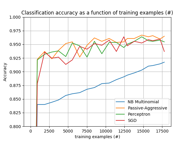
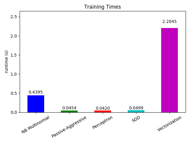
Now looking at the computation time of the different parts, we see that the
vectorization is much more expensive than learning itself. From the different
algorithms, MultinomialNB is the most expensive, but its overhead can be
mitigated by increasing the size of the mini-batches (exercise: change
minibatch_size to 100 and 10000 in the program and compare).
6.1.1.5. Notes
| [1] | Depending on the algorithm the mini-batch size can influence results or not. SGD*, PassiveAggressive*, and discrete NaiveBayes are truly online and are not affected by batch size. Conversely, MiniBatchKMeans convergence rate is affected by the batch size. Also, its memory footprint can vary dramatically with batch size. |
6.2. Computational Performance
For some applications the performance (mainly latency and throughput at prediction time) of estimators is crucial. It may also be of interest to consider the training throughput but this is often less important in a production setup (where it often takes place offline).
We will review here the orders of magnitude you can expect from a number of scikit-learn estimators in different contexts and provide some tips and tricks for overcoming performance bottlenecks.
Prediction latency is measured as the elapsed time necessary to make a prediction (e.g. in micro-seconds). Latency is often viewed as a distribution and operations engineers often focus on the latency at a given percentile of this distribution (e.g. the 90 percentile).
Prediction throughput is defined as the number of predictions the software can deliver in a given amount of time (e.g. in predictions per second).
An important aspect of performance optimization is also that it can hurt prediction accuracy. Indeed, simpler models (e.g. linear instead of non-linear, or with fewer parameters) often run faster but are not always able to take into account the same exact properties of the data as more complex ones.
6.2.1. Prediction Latency
One of the most straight-forward concerns one may have when using/choosing a machine learning toolkit is the latency at which predictions can be made in a production environment.
- The main factors that influence the prediction latency are
- Number of features
- Input data representation and sparsity
- Model complexity
- Feature extraction
A last major parameter is also the possibility to do predictions in bulk or one-at-a-time mode.
6.2.1.1. Bulk versus Atomic mode
In general doing predictions in bulk (many instances at the same time) is more efficient for a number of reasons (branching predictability, CPU cache, linear algebra libraries optimizations etc.). Here we see on a setting with few features that independently of estimator choice the bulk mode is always faster, and for some of them by 1 to 2 orders of magnitude:

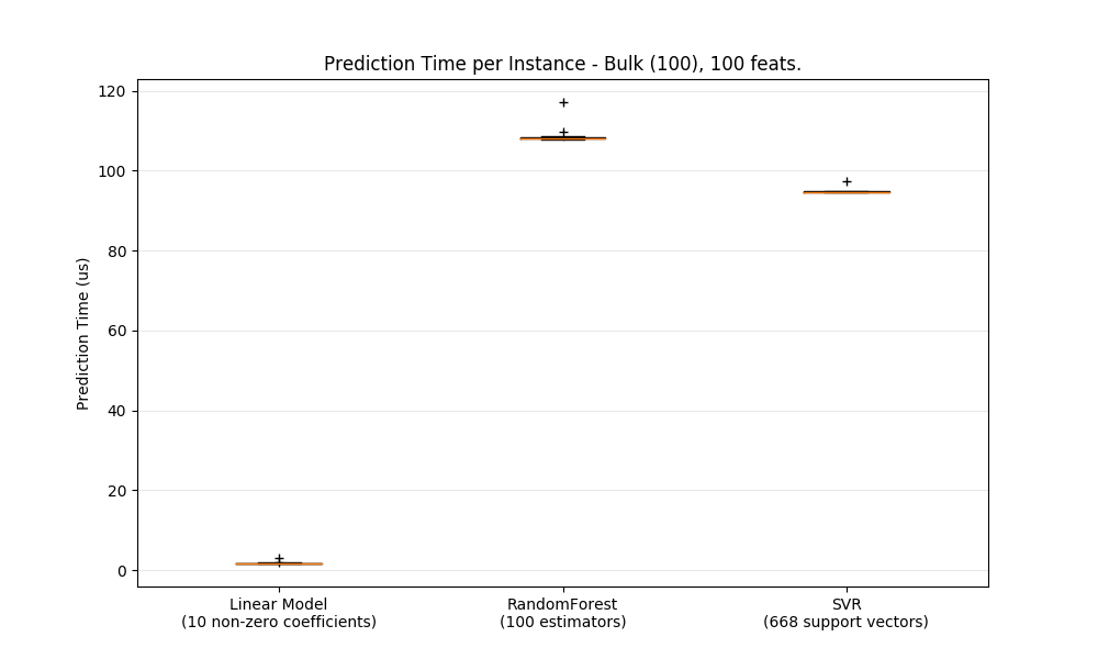
To benchmark different estimators for your case you can simply change the
n_features parameter in this example:
Prediction Latency. This should give
you an estimate of the order of magnitude of the prediction latency.
6.2.1.2. Configuring Scikit-learn for reduced validation overhead
Scikit-learn does some validation on data that increases the overhead per
call to predict and similar functions. In particular, checking that
features are finite (not NaN or infinite) involves a full pass over the
data. If you ensure that your data is acceptable, you may suppress
checking for finiteness by setting the environment variable
SKLEARN_ASSUME_FINITE to a non-empty string before importing
scikit-learn, or configure it in Python with sklearn.set_config.
For more control than these global settings, a config_context
allows you to set this configuration within a specified context:
>>> import sklearn
>>> with sklearn.config_context(assume_finite=True):
...     pass  # do learning/prediction here with reduced validation
Note that this will affect all uses of
sklearn.utils.assert_all_finite within the context.
6.2.1.3. Influence of the Number of Features
Obviously when the number of features increases so does the memory consumption of each example. Indeed, for a matrix of \(M\) instances with \(N\) features, the space complexity is in \(O(NM)\). From a computing perspective it also means that the number of basic operations (e.g., multiplications for vector-matrix products in linear models) increases too. Here is a graph of the evolution of the prediction latency with the number of features:
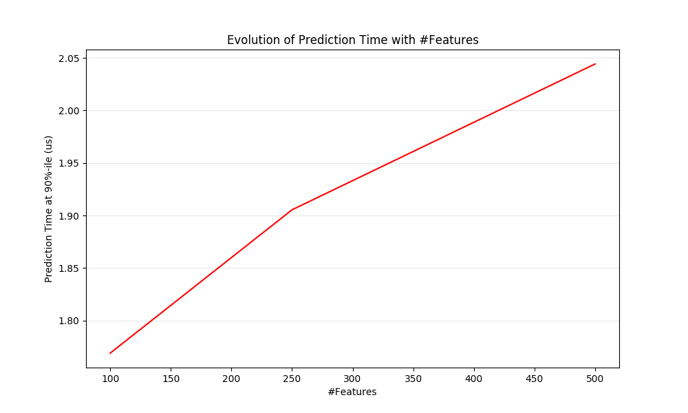
Overall you can expect the prediction time to increase at least linearly with the number of features (non-linear cases can happen depending on the global memory footprint and estimator).
6.2.1.4. Influence of the Input Data Representation
Scipy provides sparse matrix data structures which are optimized for storing sparse data. The main feature of sparse formats is that you don’t store zeros so if your data is sparse then you use much less memory. A non-zero value in a sparse (CSR or CSC) representation will only take on average one 32bit integer position + the 64 bit floating point value + an additional 32bit per row or column in the matrix. Using sparse input on a dense (or sparse) linear model can speedup prediction by quite a bit as only the non zero valued features impact the dot product and thus the model predictions. Hence if you have 100 non zeros in 1e6 dimensional space, you only need 100 multiply and add operation instead of 1e6.
Calculation over a dense representation, however, may leverage highly optimised vector operations and multithreading in BLAS, and tends to result in fewer CPU cache misses. So the sparsity should typically be quite high (10% non-zeros max, to be checked depending on the hardware) for the sparse input representation to be faster than the dense input representation on a machine with many CPUs and an optimized BLAS implementation.
Here is sample code to test the sparsity of your input:
def sparsity_ratio(X):
    return 1.0 - np.count_nonzero(X) / float(X.shape[0] * X.shape[1])
print("input sparsity ratio:", sparsity_ratio(X))
As a rule of thumb you can consider that if the sparsity ratio is greater
than 90% you can probably benefit from sparse formats. Check Scipy’s sparse
matrix formats documentation
for more information on how to build (or convert your data to) sparse matrix
formats. Most of the time the CSR and CSC formats work best.
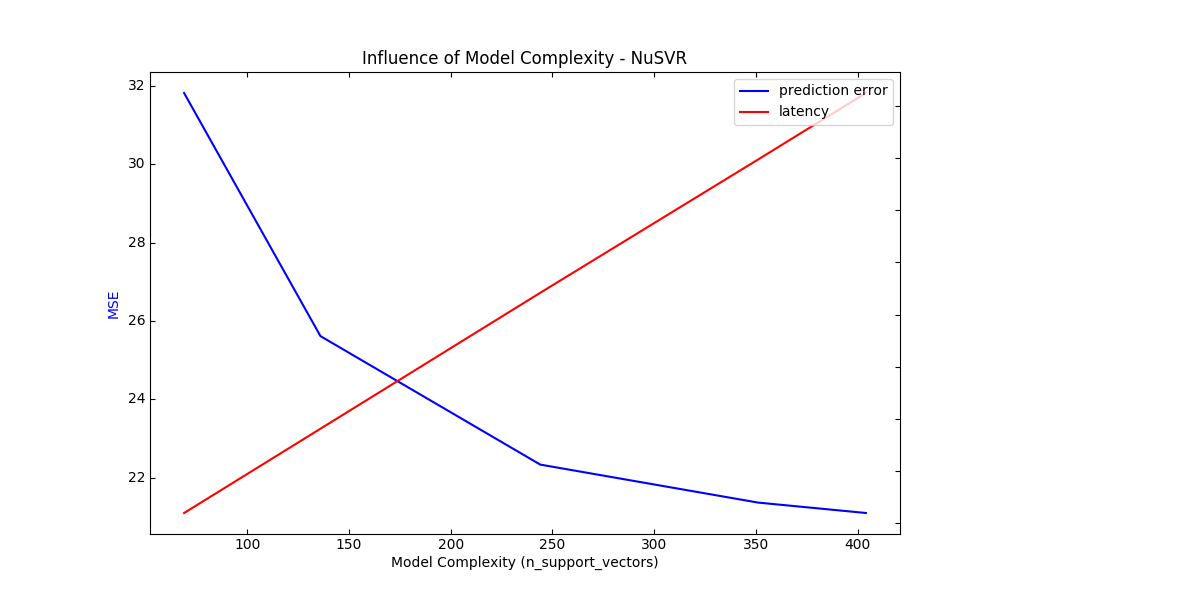
6.2.1.5. Influence of the Model Complexity
Generally speaking, when model complexity increases, predictive power and latency are supposed to increase. Increasing predictive power is usually interesting, but for many applications we would better not increase prediction latency too much. We will now review this idea for different families of supervised models.
For sklearn.linear_model (e.g. Lasso, ElasticNet,
SGDClassifier/Regressor, Ridge & RidgeClassifier,
PassiveAggressiveClassifier/Regressor, LinearSVC, LogisticRegression…) the
decision function that is applied at prediction time is the same (a dot product)
, so latency should be equivalent.
Here is an example using
sklearn.linear_model.stochastic_gradient.SGDClassifier with the
elasticnet penalty. The regularization strength is globally controlled by
the alpha parameter. With a sufficiently high alpha,
one can then increase the l1_ratio parameter of elasticnet to
enforce various levels of sparsity in the model coefficients. Higher sparsity
here is interpreted as less model complexity as we need fewer coefficients to
describe it fully. Of course sparsity influences in turn the prediction time
as the sparse dot-product takes time roughly proportional to the number of
non-zero coefficients.

For the sklearn.svm family of algorithms with a non-linear kernel,
the latency is tied to the number of support vectors (the fewer the faster).
Latency and throughput should (asymptotically) grow linearly with the number
of support vectors in a SVC or SVR model. The kernel will also influence the
latency as it is used to compute the projection of the input vector once per
support vector. In the following graph the nu parameter of
sklearn.svm.classes.NuSVR was used to influence the number of
support vectors.
For sklearn.ensemble of trees (e.g. RandomForest, GBT,
ExtraTrees etc) the number of trees and their depth play the most
important role. Latency and throughput should scale linearly with the number
of trees. In this case we used directly the n_estimators parameter of
sklearn.ensemble.gradient_boosting.GradientBoostingRegressor.
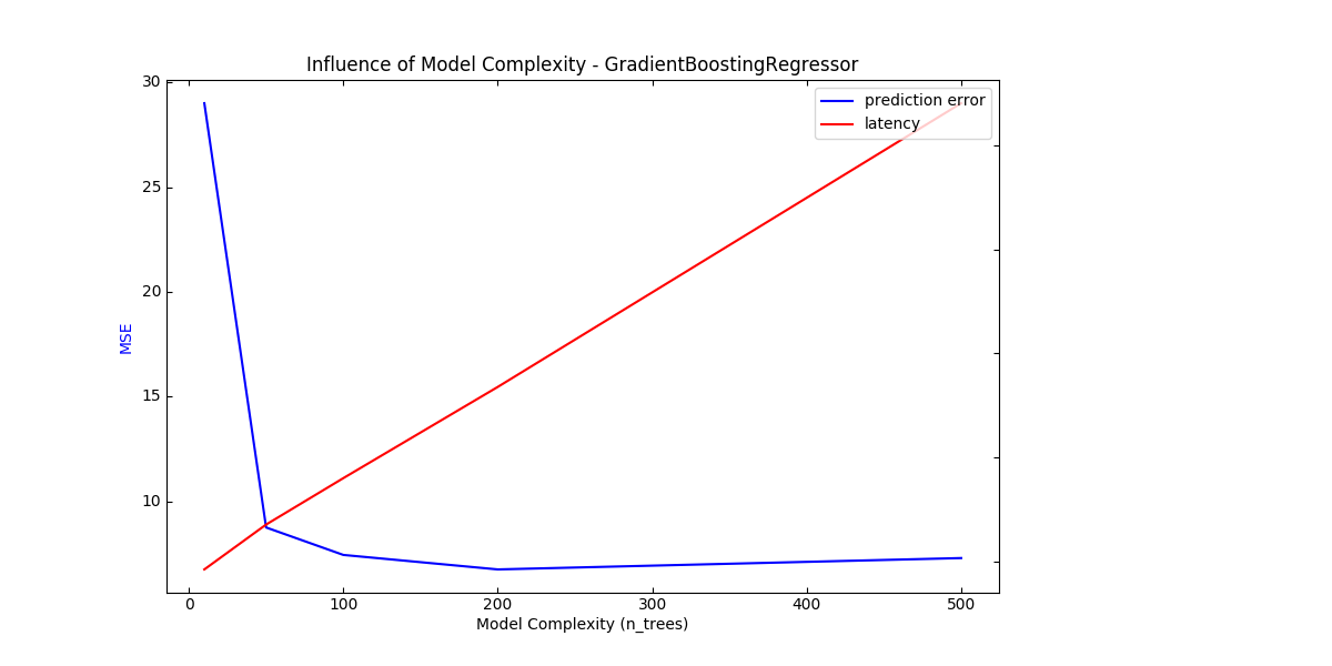
In any case be warned that decreasing model complexity can hurt accuracy as mentioned above. For instance a non-linearly separable problem can be handled with a speedy linear model but prediction power will very likely suffer in the process.
6.2.1.6. Feature Extraction Latency
Most scikit-learn models are usually pretty fast as they are implemented either with compiled Cython extensions or optimized computing libraries. On the other hand, in many real world applications the feature extraction process (i.e. turning raw data like database rows or network packets into numpy arrays) governs the overall prediction time. For example on the Reuters text classification task the whole preparation (reading and parsing SGML files, tokenizing the text and hashing it into a common vector space) is taking 100 to 500 times more time than the actual prediction code, depending on the chosen model.
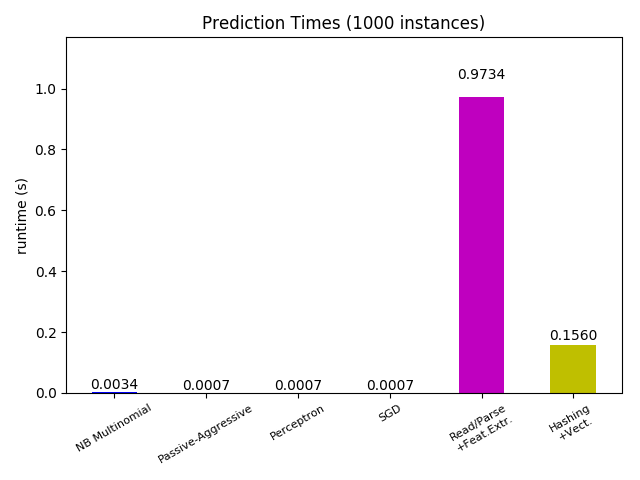
In many cases it is thus recommended to carefully time and profile your feature extraction code as it may be a good place to start optimizing when your overall latency is too slow for your application.
6.2.2. Prediction Throughput
Another important metric to care about when sizing production systems is the throughput i.e. the number of predictions you can make in a given amount of time. Here is a benchmark from the Prediction Latency example that measures this quantity for a number of estimators on synthetic data:
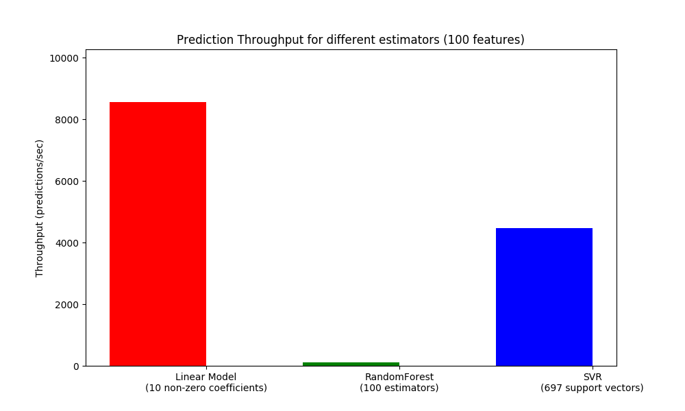
These throughputs are achieved on a single process. An obvious way to increase the throughput of your application is to spawn additional instances (usually processes in Python because of the GIL) that share the same model. One might also add machines to spread the load. A detailed explanation on how to achieve this is beyond the scope of this documentation though.
6.2.3. Tips and Tricks
6.2.3.1. Linear algebra libraries
As scikit-learn relies heavily on Numpy/Scipy and linear algebra in general it makes sense to take explicit care of the versions of these libraries. Basically, you ought to make sure that Numpy is built using an optimized BLAS / LAPACK library.
Not all models benefit from optimized BLAS and Lapack implementations. For
instance models based on (randomized) decision trees typically do not rely on
BLAS calls in their inner loops, nor do kernel SVMs (SVC, SVR,
NuSVC, NuSVR). On the other hand a linear model implemented with a
BLAS DGEMM call (via numpy.dot) will typically benefit hugely from a tuned
BLAS implementation and lead to orders of magnitude speedup over a
non-optimized BLAS.
You can display the BLAS / LAPACK implementation used by your NumPy / SciPy / scikit-learn install with the following commands:
from numpy.distutils.system_info import get_info
print(get_info('blas_opt'))
print(get_info('lapack_opt'))
- Optimized BLAS / LAPACK implementations include:
- Atlas (need hardware specific tuning by rebuilding on the target machine)
- OpenBLAS
- MKL
- Apple Accelerate and vecLib frameworks (OSX only)
More information can be found on the Scipy install page and in this blog post from Daniel Nouri which has some nice step by step install instructions for Debian / Ubuntu.
Warning
Multithreaded BLAS libraries sometimes conflict with Python’s
multiprocessing module, which is used by e.g. GridSearchCV and
most other estimators that take an n_jobs argument (with the exception
of SGDClassifier, SGDRegressor, Perceptron,
PassiveAggressiveClassifier and tree-based methods such as random
forests). This is true of Apple’s Accelerate and OpenBLAS when built with
OpenMP support.
Besides scikit-learn, NumPy and SciPy also use BLAS internally, as explained earlier.
If you experience hanging subprocesses with n_jobs>1 or n_jobs=-1,
make sure you have a single-threaded BLAS library, or set n_jobs=1,
or upgrade to Python 3.4 which has a new version of multiprocessing
that should be immune to this problem.
6.2.3.2. Limiting Working Memory
Some calculations when implemented using standard numpy vectorized operations
involve using a large amount of temporary memory. This may potentially exhaust
system memory. Where computations can be performed in fixed-memory chunks, we
attempt to do so, and allow the user to hint at the maximum size of this
working memory (defaulting to 1GB) using sklearn.set_config or
config_context. The following suggests to limit temporary working
memory to 128 MiB:
>>> import sklearn
>>> with sklearn.config_context(working_memory=128):
...     pass  # do chunked work here
An example of a chunked operation adhering to this setting is
metric.pairwise_distances_chunked, which facilitates computing
row-wise reductions of a pairwise distance matrix.
6.2.3.3. Model Compression
Model compression in scikit-learn only concerns linear models for the moment. In this context it means that we want to control the model sparsity (i.e. the number of non-zero coordinates in the model vectors). It is generally a good idea to combine model sparsity with sparse input data representation.
Here is sample code that illustrates the use of the sparsify() method:
clf = SGDRegressor(penalty='elasticnet', l1_ratio=0.25)
clf.fit(X_train, y_train).sparsify()
clf.predict(X_test)
In this example we prefer the elasticnet penalty as it is often a good
compromise between model compactness and prediction power. One can also
further tune the l1_ratio parameter (in combination with the
regularization strength alpha) to control this tradeoff.
A typical benchmark on synthetic data yields a >30% decrease in latency when both the model and input are sparse (with 0.000024 and 0.027400 non-zero coefficients ratio respectively). Your mileage may vary depending on the sparsity and size of your data and model. Furthermore, sparsifying can be very useful to reduce the memory usage of predictive models deployed on production servers.
6.2.3.4. Model Reshaping
Model reshaping consists in selecting only a portion of the available features
to fit a model. In other words, if a model discards features during the
learning phase we can then strip those from the input. This has several
benefits. Firstly it reduces memory (and therefore time) overhead of the
model itself. It also allows to discard explicit
feature selection components in a pipeline once we know which features to
keep from a previous run. Finally, it can help reduce processing time and I/O
usage upstream in the data access and feature extraction layers by not
collecting and building features that are discarded by the model. For instance
if the raw data come from a database, it can make it possible to write simpler
and faster queries or reduce I/O usage by making the queries return lighter
records.
At the moment, reshaping needs to be performed manually in scikit-learn.
In the case of sparse input (particularly in CSR format), it is generally
sufficient to not generate the relevant features, leaving their columns empty.
6.3. Parallelism, resource management, and configuration
6.3.1. Parallel and distributed computing
Scikit-learn uses the joblib library to enable parallel computing inside its estimators. See the joblib documentation for the switches to control parallel computing.
Note that, by default, scikit-learn uses its embedded (vendored) version of joblib. A configuration switch (documented below) controls this behavior.
6.3.2. Configuration switches
6.3.2.1. Python runtime
sklearn.set_config controls the following behaviors:
| assume_finite: | used to skip validation, which enables faster computations but may lead to segmentation faults if the data contains NaNs. |
|---|---|
| working_memory: | the optimal size of temporary arrays used by some algoritms. |
6.3.2.2. Environment variables
These environment variables should be set before importing scikit-learn.
| SKLEARN_SITE_JOBLIB: | |
|---|---|
| When this environment variable is set to a non zero value, scikit-learn uses the site joblib rather than its vendored version. Consequently, joblib must be installed for scikit-learn to run. Note that using the site joblib is at your own risks: the versions of scikit-learn and joblib need to be compatible. Currently, joblib 0.11+ is supported. In addition, dumps from joblib.Memory might be incompatible, and you might loose some caches and have to redownload some datasets. | |
| SKLEARN_ASSUME_FINITE: | |
Sets the default value for the assume_finite argument of
sklearn.set_config. |
|
| SKLEARN_WORKING_MEMORY: | |
Sets the default value for the working_memory argument of
sklearn.set_config. |
|
| SKLEARN_SEED: | Sets the seed of the global random generator when running the tests, for reproducibility. |
| SKLEARN_SKIP_NETWORK_TESTS: | |
| When this environment variable is set to a non zero value, the tests that need network access are skipped. | |