sklearn.discriminant_analysis.LinearDiscriminantAnalysis
-
class
sklearn.discriminant_analysis.LinearDiscriminantAnalysis(solver='svd', shrinkage=None, priors=None, n_components=None, store_covariance=False, tol=0.0001)[source]¶ Linear Discriminant Analysis
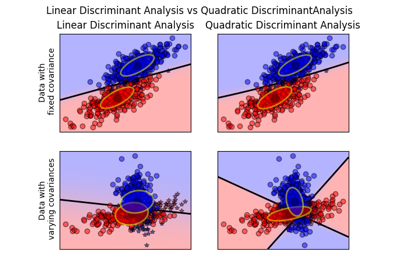
A classifier with a linear decision boundary, generated by fitting class conditional densities to the data and using Bayes’ rule.
The model fits a Gaussian density to each class, assuming that all classes share the same covariance matrix.
The fitted model can also be used to reduce the dimensionality of the input by projecting it to the most discriminative directions.
New in version 0.17: LinearDiscriminantAnalysis.
Read more in the User Guide.
Parameters: - solver : string, optional
- Solver to use, possible values:
- ‘svd’: Singular value decomposition (default). Does not compute the covariance matrix, therefore this solver is recommended for data with a large number of features.
- ‘lsqr’: Least squares solution, can be combined with shrinkage.
- ‘eigen’: Eigenvalue decomposition, can be combined with shrinkage.
- shrinkage : string or float, optional
- Shrinkage parameter, possible values:
- None: no shrinkage (default).
- ‘auto’: automatic shrinkage using the Ledoit-Wolf lemma.
- float between 0 and 1: fixed shrinkage parameter.
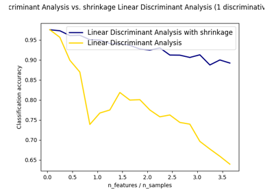
Note that shrinkage works only with ‘lsqr’ and ‘eigen’ solvers.
- priors : array, optional, shape (n_classes,)
Class priors.
- n_components : int, optional
Number of components (< n_classes - 1) for dimensionality reduction.
- store_covariance : bool, optional
Additionally compute class covariance matrix (default False), used only in ‘svd’ solver.
New in version 0.17.
- tol : float, optional, (default 1.0e-4)
Threshold used for rank estimation in SVD solver.
New in version 0.17.
Attributes: - coef_ : array, shape (n_features,) or (n_classes, n_features)
Weight vector(s).
- intercept_ : array, shape (n_features,)
Intercept term.
- covariance_ : array-like, shape (n_features, n_features)
Covariance matrix (shared by all classes).
- explained_variance_ratio_ : array, shape (n_components,)
Percentage of variance explained by each of the selected components. If
n_componentsis not set then all components are stored and the sum of explained variances is equal to 1.0. Only available when eigen or svd solver is used.- means_ : array-like, shape (n_classes, n_features)
Class means.
- priors_ : array-like, shape (n_classes,)
Class priors (sum to 1).
- scalings_ : array-like, shape (rank, n_classes - 1)
Scaling of the features in the space spanned by the class centroids.
- xbar_ : array-like, shape (n_features,)
Overall mean.
- classes_ : array-like, shape (n_classes,)
Unique class labels.
See also
sklearn.discriminant_analysis.QuadraticDiscriminantAnalysis- Quadratic Discriminant Analysis
Notes
The default solver is ‘svd’. It can perform both classification and transform, and it does not rely on the calculation of the covariance matrix. This can be an advantage in situations where the number of features is large. However, the ‘svd’ solver cannot be used with shrinkage.
The ‘lsqr’ solver is an efficient algorithm that only works for classification. It supports shrinkage.
The ‘eigen’ solver is based on the optimization of the between class scatter to within class scatter ratio. It can be used for both classification and transform, and it supports shrinkage. However, the ‘eigen’ solver needs to compute the covariance matrix, so it might not be suitable for situations with a high number of features.
Examples
>>> import numpy as np
>>> from sklearn.discriminant_analysis import LinearDiscriminantAnalysis
>>> X = np.array([[-1, -1], [-2, -1], [-3, -2], [1, 1], [2, 1], [3, 2]])
>>> y = np.array([1, 1, 1, 2, 2, 2])
>>> clf = LinearDiscriminantAnalysis()
>>> clf.fit(X, y)
LinearDiscriminantAnalysis(n_components=None, priors=None, shrinkage=None,
              solver='svd', store_covariance=False, tol=0.0001)
>>> print(clf.predict([[-0.8, -1]]))
[1]
Methods
decision_function(X)Predict confidence scores for samples. fit(X, y)Fit LinearDiscriminantAnalysis model according to the given fit_transform(X[, y])Fit to data, then transform it. get_params([deep])Get parameters for this estimator. predict(X)Predict class labels for samples in X. predict_log_proba(X)Estimate log probability. predict_proba(X)Estimate probability. score(X, y[, sample_weight])Returns the mean accuracy on the given test data and labels. set_params(**params)Set the parameters of this estimator. transform(X)Project data to maximize class separation. -
__init__(solver='svd', shrinkage=None, priors=None, n_components=None, store_covariance=False, tol=0.0001)[source]¶ Initialize self. See help(type(self)) for accurate signature.
-
decision_function(X)[source]¶ Predict confidence scores for samples.
The confidence score for a sample is the signed distance of that sample to the hyperplane.
Parameters: - X : array_like or sparse matrix, shape (n_samples, n_features)
Samples.
Returns: - array, shape=(n_samples,) if n_classes == 2 else (n_samples, n_classes)
Confidence scores per (sample, class) combination. In the binary case, confidence score for self.classes_[1] where >0 means this class would be predicted.
-
fit(X, y)[source]¶ - Fit LinearDiscriminantAnalysis model according to the given
training data and parameters.
Changed in version 0.19: store_covariance has been moved to main constructor.
Changed in version 0.19: tol has been moved to main constructor.
Parameters: - X : array-like, shape (n_samples, n_features)
Training data.
- y : array, shape (n_samples,)
Target values.
-
fit_transform(X, y=None, **fit_params)[source]¶ Fit to data, then transform it.
Fits transformer to X and y with optional parameters fit_params and returns a transformed version of X.
Parameters: - X : numpy array of shape [n_samples, n_features]
Training set.
- y : numpy array of shape [n_samples]
Target values.
Returns: - X_new : numpy array of shape [n_samples, n_features_new]
Transformed array.
-
get_params(deep=True)[source]¶ Get parameters for this estimator.
Parameters: - deep : boolean, optional
If True, will return the parameters for this estimator and contained subobjects that are estimators.
Returns: - params : mapping of string to any
Parameter names mapped to their values.
-
predict(X)[source]¶ Predict class labels for samples in X.
Parameters: - X : array_like or sparse matrix, shape (n_samples, n_features)
Samples.
Returns: - C : array, shape [n_samples]
Predicted class label per sample.
-
predict_log_proba(X)[source]¶ Estimate log probability.
Parameters: - X : array-like, shape (n_samples, n_features)
Input data.
Returns: - C : array, shape (n_samples, n_classes)
Estimated log probabilities.
-
predict_proba(X)[source]¶ Estimate probability.
Parameters: - X : array-like, shape (n_samples, n_features)
Input data.
Returns: - C : array, shape (n_samples, n_classes)
Estimated probabilities.
-
score(X, y, sample_weight=None)[source]¶ Returns the mean accuracy on the given test data and labels.
In multi-label classification, this is the subset accuracy which is a harsh metric since you require for each sample that each label set be correctly predicted.
Parameters: - X : array-like, shape = (n_samples, n_features)
Test samples.
- y : array-like, shape = (n_samples) or (n_samples, n_outputs)
True labels for X.
- sample_weight : array-like, shape = [n_samples], optional
Sample weights.
Returns: - score : float
Mean accuracy of self.predict(X) wrt. y.
-
set_params(**params)[source]¶ Set the parameters of this estimator.
The method works on simple estimators as well as on nested objects (such as pipelines). The latter have parameters of the form
<component>__<parameter>so that it’s possible to update each component of a nested object.Returns: - self