Histogram Equalization

Prev Tutorial: Affine Transformations

Next Tutorial: Histogram Calculation

Goal

In this tutorial you will learn:

• What an image histogram is and why it is useful
• To equalize histograms of images by using the OpenCV function cv::equalizeHist

Theory

What is an Image Histogram?

• It is a graphical representation of the intensity distribution of an image.
• It quantifies the number of pixels for each intensity value considered.

What is Histogram Equalization?

• It is a method that improves the contrast in an image, in order to stretch out the intensity range (see also the corresponding Wikipedia entry).
• To make it clearer, from the image above, you can see that the pixels seem clustered around the middle of the available range of intensities. What Histogram Equalization does is to stretch out this range. Take a look at the figure below: The green circles indicate the underpopulated intensities. After applying the equalization, we get an histogram like the figure in the center. The resulting image is shown in the picture at right.

How does it work?

• Equalization implies mapping one distribution (the given histogram) to another distribution (a wider and more uniform distribution of intensity values) so the intensity values are spread over the whole range.

• To accomplish the equalization effect, the remapping should be the cumulative distribution function (cdf) (more details, refer to Learning OpenCV). For the histogram $H(i)$, its cumulative distribution $H^{'}(i)$ is:

  $$H^{'}(i) = \sum_{0 \le j < i} H(j)$$

  To use this as a remapping function, we have to normalize $H^{'}(i)$ such that the maximum value is 255 ( or the maximum value for the intensity of the image ). From the example above, the cumulative function is:

  

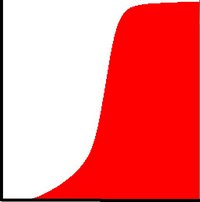
• Finally, we use a simple remapping procedure to obtain the intensity values of the equalized image:

  $$equalized( x, y ) = H^{'}( src(x,y) )$$

Code

C++JavaPython

• What does this program do?
  • Loads an image
  • Convert the original image to grayscale
  • Equalize the Histogram by using the OpenCV function cv::equalizeHist
  • Display the source and equalized images in a window.

[block]

C++

• Downloadable code: Click here

• Code at glance:

  
  #include "opencv2/imgcodecs.hpp"
  #include "opencv2/highgui.hpp"
  #include "opencv2/imgproc.hpp"
  #include <iostream>
  
  using namespace cv;
  using namespace std;
  
  int main( int argc, char** argv )
  {
      CommandLineParser parser( argc, argv, "{@input | ../data/lena.jpg | input image}" );
      Mat src = imread( parser.get<String>( "@input" ), IMREAD_COLOR );
      if( src.empty() )
      {
          cout << "Could not open or find the image!\n" << endl;
          cout << "Usage: " << argv[0] << " <Input image>" << endl;
          return -1;
      }
  
      cvtColor( src, src, COLOR_BGR2GRAY );
  
      Mat dst;
      equalizeHist( src, dst );
  
      imshow( "Source image", src );
      imshow( "Equalized Image", dst );
  
      waitKey();
  
      return 0;
  
  }

  [block]

[block]

Java

• Downloadable code: Click here

• Code at glance:

  import org.opencv.core.Core;
  import org.opencv.core.Mat;
  import org.opencv.highgui.HighGui;
  import org.opencv.imgcodecs.Imgcodecs;
  import org.opencv.imgproc.Imgproc;
  
  class EqualizeHist {
      public void run(String[] args) {
          String filename = args.length > 0 ? args[0] : "../data/lena.jpg";
          Mat src = Imgcodecs.imread(filename);
          if (src.empty()) {
              System.err.println("Cannot read image: " + filename);
              System.exit(0);
          }
  
          Imgproc.cvtColor(src, src, Imgproc.COLOR_BGR2GRAY);
  
          Mat dst = new Mat();
          Imgproc.equalizeHist( src, dst );
  
          HighGui.imshow( "Source image", src );
          HighGui.imshow( "Equalized Image", dst );
  
          HighGui.waitKey(0);
  
          System.exit(0);
      }
  }
  
  public class EqualizeHistDemo {
  
      public static void main(String[] args) {
          // Load the native OpenCV library
          System.loadLibrary(Core.NATIVE_LIBRARY_NAME);
  
          new EqualizeHist().run(args);
      }
  
  }

  [block]

[block]

Python

• Downloadable code: Click here

• Code at glance:

  from __future__ import print_function
  import cv2 as cv
  import argparse
  
  ## [Load image]
  parser = argparse.ArgumentParser(description='Code for Histogram Equalization tutorial.')
  parser.add_argument('--input', help='Path to input image.', default='lena.jpg')
  args = parser.parse_args()
  
  src = cv.imread(cv.samples.findFile(args.input))
  if src is None:
      print('Could not open or find the image:', args.input)
      exit(0)
  ## [Load image]
  
  ## [Convert to grayscale]
  src = cv.cvtColor(src, cv.COLOR_BGR2GRAY)
  ## [Convert to grayscale]
  
  ## [Apply Histogram Equalization]
  dst = cv.equalizeHist(src)
  ## [Apply Histogram Equalization]
  
  ## [Display results]
  cv.imshow('Source image', src)
  cv.imshow('Equalized Image', dst)
  ## [Display results]
  
  ## [Wait until user exits the program]
  cv.waitKey()
  ## [Wait until user exits the program]

  [block]

Explanation

C++JavaPython

• Load the source image:

[block]

C++

    CommandLineParser parser( argc, argv, "{@input | ../data/lena.jpg | input image}" );
    Mat src = imread( parser.get<String>( "@input" ), IMREAD_COLOR );
    if( src.empty() )
    {
        cout << "Could not open or find the image!\n" << endl;
        cout << "Usage: " << argv[0] << " <Input image>" << endl;
        return -1;
    }

[block]

[block]

Java

        String filename = args.length > 0 ? args[0] : "../data/lena.jpg";
        Mat src = Imgcodecs.imread(filename);
        if (src.empty()) {
            System.err.println("Cannot read image: " + filename);
            System.exit(0);
        }

[block]

[block]

Python

parser = argparse.ArgumentParser(description='Code for Histogram Equalization tutorial.')
parser.add_argument('--input', help='Path to input image.', default='lena.jpg')
args = parser.parse_args()

src = cv.imread(cv.samples.findFile(args.input))
if src is None:
    print('Could not open or find the image:', args.input)
    exit(0)

[block]

• Convert it to grayscale:

[block]

C++

    cvtColor( src, src, COLOR_BGR2GRAY );

[block]

[block]

Java

        Imgproc.cvtColor(src, src, Imgproc.COLOR_BGR2GRAY);

[block]

[block]

Python

src = cv.cvtColor(src, cv.COLOR_BGR2GRAY)

[block]

• Apply histogram equalization with the function cv::equalizeHist :

[block]

C++

    Mat dst;
    equalizeHist( src, dst );

[block]

[block]

Java

        Mat dst = new Mat();
        Imgproc.equalizeHist( src, dst );

[block]

[block]

Python

dst = cv.equalizeHist(src)

[block]

As it can be easily seen, the only arguments are the original image and the output (equalized) image.

• Display both images (original and equalized):

[block]

C++

    imshow( "Source image", src );
    imshow( "Equalized Image", dst );

[block]

[block]

Java

        HighGui.imshow( "Source image", src );
        HighGui.imshow( "Equalized Image", dst );

[block]

[block]

Python

cv.imshow('Source image', src)
cv.imshow('Equalized Image', dst)

[block]

• Wait until user exists the program

[block]

C++

    waitKey();

[block]

[block]

Java

        HighGui.waitKey(0);

[block]

[block]

Python

cv.waitKey()

[block]

Results

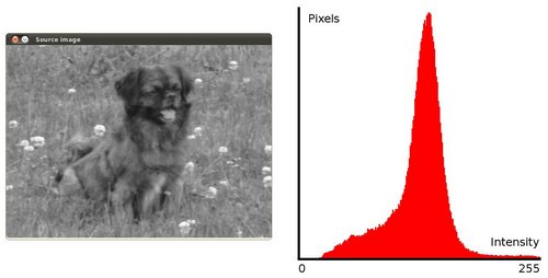
1. To appreciate better the results of equalization, let's introduce an image with not much contrast, such as:

   

   which, by the way, has this histogram:

   

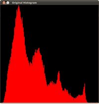
   notice that the pixels are clustered around the center of the histogram.

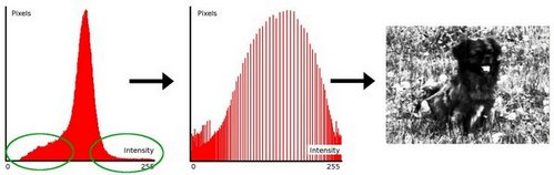
1. After applying the equalization with our program, we get this result:

   

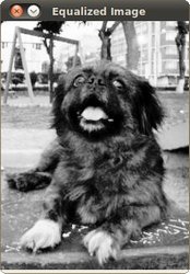
   this image has certainly more contrast. Check out its new histogram like this:

   

   Notice how the number of pixels is more distributed through the intensity range.

Note

Are you wondering how did we draw the Histogram figures shown above? Check out the following tutorial!