scipy.signal.spectrogram
- scipy.signal.spectrogram(x, fs=1.0, window=('tukey', 0.25), nperseg=256, noverlap=None, nfft=None, detrend='constant', return_onesided=True, scaling='density', axis=-1, mode='psd')[source]
Compute a spectrogram with consecutive Fourier transforms.
Spectrograms can be used as a way of visualizing the change of a nonstationary signal’s frequency content over time.
Parameters: x : array_like
Time series of measurement values
fs : float, optional
Sampling frequency of the x time series. Defaults to 1.0.
window : str or tuple or array_like, optional
Desired window to use. See get_window for a list of windows and required parameters. If window is array_like it will be used directly as the window and its length will be used for nperseg. Defaults to a Tukey window with shape parameter of 0.25.
nperseg : int, optional
Length of each segment. Defaults to 256.
noverlap : int, optional
Number of points to overlap between segments. If None, noverlap = nperseg // 8. Defaults to None.
nfft : int, optional
Length of the FFT used, if a zero padded FFT is desired. If None, the FFT length is nperseg. Defaults to None.
detrend : str or function or False, optional
return_onesided : bool, optional
If True, return a one-sided spectrum for real data. If False return a two-sided spectrum. Note that for complex data, a two-sided spectrum is always returned.
scaling : { ‘density’, ‘spectrum’ }, optional
Selects between computing the power spectral density (‘density’) where Pxx has units of V**2/Hz and computing the power spectrum (‘spectrum’) where Pxx has units of V**2, if x is measured in V and fs is measured in Hz. Defaults to ‘density’
axis : int, optional
Axis along which the spectrogram is computed; the default is over the last axis (i.e. axis=-1).
mode : str, optional
Defines what kind of return values are expected. Options are [‘psd’, ‘complex’, ‘magnitude’, ‘angle’, ‘phase’].
Returns: f : ndarray
Array of sample frequencies.
t : ndarray
Array of segment times.
Sxx : ndarray
Spectrogram of x. By default, the last axis of Sxx corresponds to the segment times.
See also
- periodogram
- Simple, optionally modified periodogram
- lombscargle
- Lomb-Scargle periodogram for unevenly sampled data
- welch
- Power spectral density by Welch’s method.
- csd
- Cross spectral density by Welch’s method.
Notes
An appropriate amount of overlap will depend on the choice of window and on your requirements. In contrast to welch’s method, where the entire data stream is averaged over, one may wish to use a smaller overlap (or perhaps none at all) when computing a spectrogram, to maintain some statistical independence between individual segments.
New in version 0.16.0.
References
[R212] Oppenheim, Alan V., Ronald W. Schafer, John R. Buck “Discrete-Time Signal Processing”, Prentice Hall, 1999. Examples
>>> from scipy import signal
>>> import matplotlib.pyplot as plt
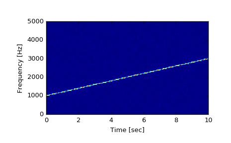
Generate a test signal, a 2 Vrms sine wave whose frequency linearly changes with time from 1kHz to 2kHz, corrupted by 0.001 V**2/Hz of white noise sampled at 10 kHz.
>>> fs = 10e3
>>> N = 1e5
>>> amp = 2 * np.sqrt(2)
>>> noise_power = 0.001 * fs / 2
>>> time = np.arange(N) / fs
>>> freq = np.linspace(1e3, 2e3, N)
>>> x = amp * np.sin(2*np.pi*freq*time)
>>> x += np.random.normal(scale=np.sqrt(noise_power), size=time.shape)
Compute and plot the spectrogram.
>>> f, t, Sxx = signal.spectrogram(x, fs)
>>> plt.pcolormesh(t, f, Sxx)
>>> plt.ylabel('Frequency [Hz]')
>>> plt.xlabel('Time [sec]')
>>> plt.show()