scipy.stats.boxcox
- scipy.stats.boxcox(x, lmbda=None, alpha=None)[source]
Return a positive dataset transformed by a Box-Cox power transformation.
Parameters: x : ndarray
Input array. Should be 1-dimensional.
lmbda : {None, scalar}, optional
If lmbda is not None, do the transformation for that value.
If lmbda is None, find the lambda that maximizes the log-likelihood function and return it as the second output argument.
alpha : {None, float}, optional
If alpha is not None, return the 100 * (1-alpha)% confidence interval for lmbda as the third output argument. Must be between 0.0 and 1.0.
Returns: boxcox : ndarray
Box-Cox power transformed array.
maxlog : float, optional
If the lmbda parameter is None, the second returned argument is the lambda that maximizes the log-likelihood function.
(min_ci, max_ci) : tuple of float, optional
If lmbda parameter is None and alpha is not None, this returned tuple of floats represents the minimum and maximum confidence limits given alpha.
See also
Notes
The Box-Cox transform is given by:
y = (x**lmbda - 1) / lmbda,  for lmbda > 0
    log(x),                  for lmbda = 0
boxcox requires the input data to be positive. Sometimes a Box-Cox transformation provides a shift parameter to achieve this; boxcox does not. Such a shift parameter is equivalent to adding a positive constant to x before calling boxcox.
The confidence limits returned when alpha is provided give the interval where:
\[\begin{split}llf(\hat{\lambda}) - llf(\lambda) < \frac{1}{2}\chi^2(1 - \alpha, 1),\end{split}\]with llf the log-likelihood function and \(\chi^2\) the chi-squared function.
References
G.E.P. Box and D.R. Cox, “An Analysis of Transformations”, Journal of the Royal Statistical Society B, 26, 211-252 (1964).
Examples
>>> from scipy import stats
>>> import matplotlib.pyplot as plt
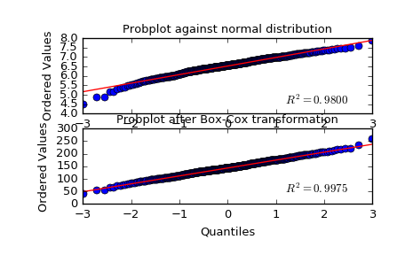
We generate some random variates from a non-normal distribution and make a probability plot for it, to show it is non-normal in the tails:
>>> fig = plt.figure()
>>> ax1 = fig.add_subplot(211)
>>> x = stats.loggamma.rvs(5, size=500) + 5
>>> prob = stats.probplot(x, dist=stats.norm, plot=ax1)
>>> ax1.set_xlabel('')
>>> ax1.set_title('Probplot against normal distribution')
We now use boxcox to transform the data so it’s closest to normal:
>>> ax2 = fig.add_subplot(212)
>>> xt, _ = stats.boxcox(x)
>>> prob = stats.probplot(xt, dist=stats.norm, plot=ax2)
>>> ax2.set_title('Probplot after Box-Cox transformation')
>>> plt.show()