scipy.stats.boxcox_normplot

scipy.stats.boxcox_normplot(x, la, lb, plot=None, N=80)

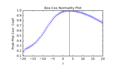
Compute parameters for a Box-Cox normality plot, optionally show it.

A Box-Cox normality plot shows graphically what the best transformation parameter is to use in boxcox to obtain a distribution that is close to normal.

Parameters:

x : array_like

Input array.

la, lb : scalar

The lower and upper bounds for the lmbda values to pass to boxcox for Box-Cox transformations. These are also the limits of the horizontal axis of the plot if that is generated.

plot : object, optional

If given, plots the quantiles and least squares fit. plot is an object that has to have methods “plot” and “text”. The matplotlib.pyplot module or a Matplotlib Axes object can be used, or a custom object with the same methods. Default is None, which means that no plot is created.

N : int, optional

Number of points on the horizontal axis (equally distributed from la to lb).

Returns:

lmbdas : ndarray

The lmbda values for which a Box-Cox transform was done.

ppcc : ndarray

Probability Plot Correlelation Coefficient, as obtained from probplot when fitting the Box-Cox transformed input x against a normal distribution.

See also

probplot, boxcox, boxcox_normmax, boxcox_llf, ppcc_max

Notes

Even if plot is given, the figure is not shown or saved by boxcox_normplot; plt.show() or plt.savefig('figname.png') should be used after calling probplot.

Examples

>>> from scipy import stats
>>> import matplotlib.pyplot as plt

Generate some non-normally distributed data, and create a Box-Cox plot:

>>> x = stats.loggamma.rvs(5, size=500) + 5
>>> fig = plt.figure()
>>> ax = fig.add_subplot(111)
>>> prob = stats.boxcox_normplot(x, -20, 20, plot=ax)

Determine and plot the optimal lmbda to transform x and plot it in the same plot:

>>> _, maxlog = stats.boxcox(x)
>>> ax.axvline(maxlog, color='r')

>>> plt.show()

(Source code)