scipy.stats.geom

scipy.stats.geom = <scipy.stats._discrete_distns.geom_gen object at 0x5987b50>

A geometric discrete random variable.

As an instance of the rv_discrete class, geom object inherits from it a collection of generic methods (see below for the full list), and completes them with details specific for this particular distribution.

Notes

The probability mass function for geom is:

geom.pmf(k) = (1-p)**(k-1)*p

for k >= 1.

geom takes p as shape parameter.

The probability mass function above is defined in the “standardized” form. To shift distribution use the loc parameter. Specifically, geom.pmf(k, p, loc) is identically equivalent to geom.pmf(k - loc, p).

Examples

>>> from scipy.stats import geom
>>> import matplotlib.pyplot as plt
>>> fig, ax = plt.subplots(1, 1)

Calculate a few first moments:

>>> p = 0.5
>>> mean, var, skew, kurt = geom.stats(p, moments='mvsk')

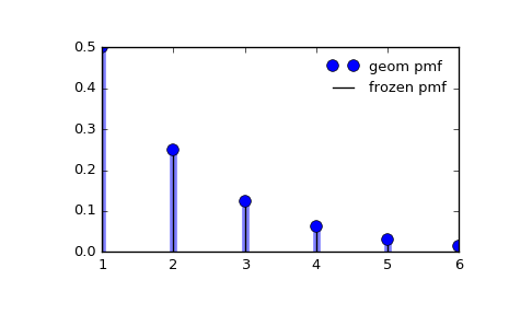
Display the probability mass function (pmf):

>>> x = np.arange(geom.ppf(0.01, p),
...               geom.ppf(0.99, p))
>>> ax.plot(x, geom.pmf(x, p), 'bo', ms=8, label='geom pmf')
>>> ax.vlines(x, 0, geom.pmf(x, p), colors='b', lw=5, alpha=0.5)

Alternatively, the distribution object can be called (as a function) to fix the shape and location. This returns a “frozen” RV object holding the given parameters fixed.

Freeze the distribution and display the frozen pmf:

>>> rv = geom(p)
>>> ax.vlines(x, 0, rv.pmf(x), colors='k', linestyles='-', lw=1,
...         label='frozen pmf')
>>> ax.legend(loc='best', frameon=False)
>>> plt.show()

(Source code)

Check accuracy of cdf and ppf:

>>> prob = geom.cdf(x, p)
>>> np.allclose(x, geom.ppf(prob, p))
True

Generate random numbers:

>>> r = geom.rvs(p, size=1000)

Methods

rvs(p, loc=0, size=1, random_state=None)	Random variates.
pmf(x, p, loc=0)	Probability mass function.
logpmf(x, p, loc=0)	Log of the probability mass function.
cdf(x, p, loc=0)	Cumulative density function.
logcdf(x, p, loc=0)	Log of the cumulative density function.
sf(x, p, loc=0)	Survival function (also defined as 1 - cdf, but sf is sometimes more accurate).
logsf(x, p, loc=0)	Log of the survival function.
ppf(q, p, loc=0)	Percent point function (inverse of cdf — percentiles).
isf(q, p, loc=0)	Inverse survival function (inverse of sf).
stats(p, loc=0, moments='mv')	Mean(‘m’), variance(‘v’), skew(‘s’), and/or kurtosis(‘k’).
entropy(p, loc=0)	(Differential) entropy of the RV.
expect(func, args=(p,), loc=0, lb=None, ub=None, conditional=False)	Expected value of a function (of one argument) with respect to the distribution.
median(p, loc=0)	Median of the distribution.
mean(p, loc=0)	Mean of the distribution.
var(p, loc=0)	Variance of the distribution.
std(p, loc=0)	Standard deviation of the distribution.
interval(alpha, p, loc=0)	Endpoints of the range that contains alpha percent of the distribution