scipy.stats.hypergeom

scipy.stats.hypergeom = <scipy.stats._discrete_distns.hypergeom_gen object at 0x5987e90>

A hypergeometric discrete random variable.

The hypergeometric distribution models drawing objects from a bin. M is the total number of objects, n is total number of Type I objects. The random variate represents the number of Type I objects in N drawn without replacement from the total population.

As an instance of the rv_discrete class, hypergeom object inherits from it a collection of generic methods (see below for the full list), and completes them with details specific for this particular distribution.

Notes

The probability mass function is defined as:

pmf(k, M, n, N) = choose(n, k) * choose(M - n, N - k) / choose(M, N),
                               for max(0, N - (M-n)) <= k <= min(n, N)

The probability mass function above is defined in the “standardized” form. To shift distribution use the loc parameter. Specifically, hypergeom.pmf(k, M, n, N, loc) is identically equivalent to hypergeom.pmf(k - loc, M, n, N).

Examples

>>> from scipy.stats import hypergeom
>>> import matplotlib.pyplot as plt

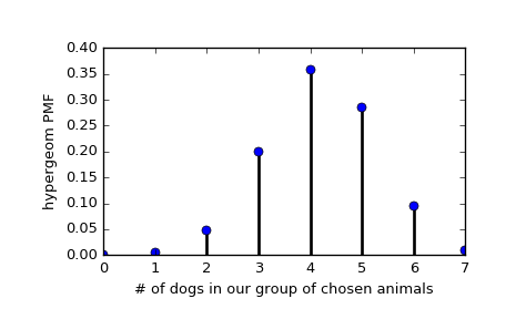
Suppose we have a collection of 20 animals, of which 7 are dogs. Then if we want to know the probability of finding a given number of dogs if we choose at random 12 of the 20 animals, we can initialize a frozen distribution and plot the probability mass function:

>>> [M, n, N] = [20, 7, 12]
>>> rv = hypergeom(M, n, N)
>>> x = np.arange(0, n+1)
>>> pmf_dogs = rv.pmf(x)

>>> fig = plt.figure()
>>> ax = fig.add_subplot(111)
>>> ax.plot(x, pmf_dogs, 'bo')
>>> ax.vlines(x, 0, pmf_dogs, lw=2)
>>> ax.set_xlabel('# of dogs in our group of chosen animals')
>>> ax.set_ylabel('hypergeom PMF')
>>> plt.show()

(Source code)

Instead of using a frozen distribution we can also use hypergeom methods directly. To for example obtain the cumulative distribution function, use:

>>> prb = hypergeom.cdf(x, M, n, N)

And to generate random numbers:

>>> R = hypergeom.rvs(M, n, N, size=10)

Methods

rvs(M, n, N, loc=0, size=1, random_state=None)	Random variates.
pmf(x, M, n, N, loc=0)	Probability mass function.
logpmf(x, M, n, N, loc=0)	Log of the probability mass function.
cdf(x, M, n, N, loc=0)	Cumulative density function.
logcdf(x, M, n, N, loc=0)	Log of the cumulative density function.
sf(x, M, n, N, loc=0)	Survival function (also defined as 1 - cdf, but sf is sometimes more accurate).
logsf(x, M, n, N, loc=0)	Log of the survival function.
ppf(q, M, n, N, loc=0)	Percent point function (inverse of cdf — percentiles).
isf(q, M, n, N, loc=0)	Inverse survival function (inverse of sf).
stats(M, n, N, loc=0, moments='mv')	Mean(‘m’), variance(‘v’), skew(‘s’), and/or kurtosis(‘k’).
entropy(M, n, N, loc=0)	(Differential) entropy of the RV.
expect(func, args=(M, n, N), loc=0, lb=None, ub=None, conditional=False)	Expected value of a function (of one argument) with respect to the distribution.
median(M, n, N, loc=0)	Median of the distribution.
mean(M, n, N, loc=0)	Mean of the distribution.
var(M, n, N, loc=0)	Variance of the distribution.
std(M, n, N, loc=0)	Standard deviation of the distribution.
interval(alpha, M, n, N, loc=0)	Endpoints of the range that contains alpha percent of the distribution