Internal documentation of the scan op
Top-level description of scan
The scan operation is meant to be able to describe symbolically loops, recurrent relations or dynamical systems. In general, we will say that the scan op implements system of equations of the following form:
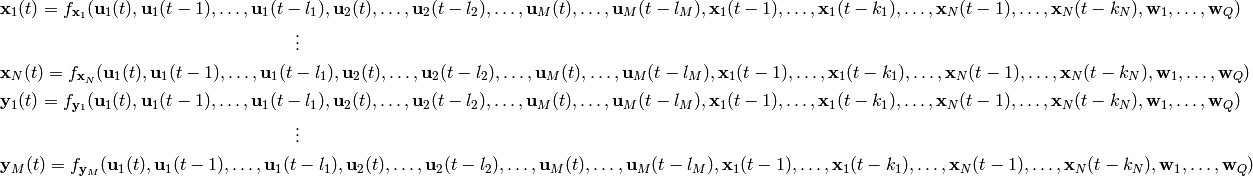
The equations describe a system evolving in time, where  represents the
current step. The system is described by inputs, states, outputs and
parameteres.
represents the
current step. The system is described by inputs, states, outputs and
parameteres.
The inputs, denoted by  are time-varying quantities,
hence indexed by . They however only influence the system, but are
not influenced by the system.
are time-varying quantities,
hence indexed by . They however only influence the system, but are
not influenced by the system.
The states  are time-varying quantities, whose value at
time depends on its (or other state) previous values as well as
the inputs and parameters. Note that the first few values of the states are
always provided, otherwise we could not imploy the recurrent equation to
generate these sequence of values without a starting point.
are time-varying quantities, whose value at
time depends on its (or other state) previous values as well as
the inputs and parameters. Note that the first few values of the states are
always provided, otherwise we could not imploy the recurrent equation to
generate these sequence of values without a starting point.
The outputs,  are outputs of the system, i.e. values that
depend on the previous values of the states and inputs. The difference
between outputs and states is that outputs do not feed back into the system.
are outputs of the system, i.e. values that
depend on the previous values of the states and inputs. The difference
between outputs and states is that outputs do not feed back into the system.
The parameters  are fixed quantities that are re-used at
every time step of the evolution of the system.
are fixed quantities that are re-used at
every time step of the evolution of the system.
Each of the equations above are implemented by the inner function of scan. You can think of the inner function as a theano function that gets executed at each step to get the new values. This inner function should not be confused with the constructive function, which is what the user gives to the scan function. The constructive function is used to construct the computational graph that is afterwards compiled into the inner function.
Naming conventions
input_statewill stand for a state, when it is
provided as an input to the recurrent formula (the inner function) that
will generate the new value of the stateoutput_statewill stand for a state when it refers
to the result of the recurrent formula (the output of the inner function)outputwill stand for an outputinputwill be an inputparameterwill stand for a parameter tensor that stays
constant at each step of the inner functionnon_numeric_input_statewill stand for states that are not numeric in nature, more specifically random states, when they are provided as an input. The same holds fornon_numeric_output_state.tis the time index (the current step in the evolution of the system).Tis the total number of steps in the evolution of the system.- the suffix
_slicesadded to eitherxoruwill mean the list of variables representing slices of states or inputs. These are the arguments given to the constructive function of scan (see above). - the suffix
_inneradded tox,y,xy,u,worzwill mean the variables representing the state/output/input/weights in the inner function - the suffix
_outeradded tox,y,xy,u,worzwill mean the variables representing the state/output/input/weights in the main computational graph (the one containing the scan op).
Files
The implementation of scan is spread over several files. The different files, and section of the code they deal with, are :
scan.pyimplements thescanfunction. Thescanfunction arranges the arguments of scan correctly, constructs the scan op and afterwards calls the constructed scan op on the arguments. This function takes care of figuring out missing inputs and shared variables.scan_op.pyimplements thescanOpclass. ThescanOprespects theOpinterface, and contains most of the logic of the scan operator.scan_utils.pycontains several helpful functions used through out the other files that are specific of the scan operator.scan_views.pycontains different views of the scan op that have simpler and easier signatures to be used in specific cases.scan_opt.pycontains the list of all optimizations for the scan operator.
The logical flow
First the scan arguments are parsed by the function canonical_arguments,
that wraps them into lists and adds default values for the arguments. One
important step that happens in this function is that the inputs arguments
are converted such that they all have a single tap, namely 0. For example
if you have [{'input':u, 'taps':[0, 4]}] as the list of inputs arguments
to scan, it gets converted into [{'input':u, 'taps':[0]}, {'input':u[4:],
'taps':[0]}].
The second step is to check if n_steps is a constant and has the value 1
or -1. If that is true then the function one_step_scan is called which
unwraps the computation of the inner function into the outer graph without
adding any scan op in the graph.