nnet – Ops for neural networks
-
tensor.nnet.sigmoid(x)¶ - Returns the standard sigmoid nonlinearity applied to x
Parameters: x - symbolic Tensor (or compatible)
Return type: same as x
Returns: element-wise sigmoid:
 .
.note: see
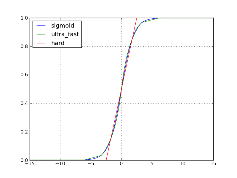
ultra_fast_sigmoid()orhard_sigmoid()for faster versions. Speed comparison for 100M float64 elements on a Core2 Duo @ 3.16 GHz:- hard_sigmoid: 1.0s
- ultra_fast_sigmoid: 1.3s
- sigmoid (with amdlibm): 2.3s
- sigmoid (without amdlibm): 3.7s
Precision: sigmoid(without or without amdlibm) > ultra_fast_sigmoid > hard_sigmoid.
Example:
import theano.tensor as T

x, y, b = T.dvectors('x', 'y', 'b')
W = T.dmatrix('W')
y = T.nnet.sigmoid(T.dot(W, x) + b)
Note
The underlying code will return an exact 0 or 1 if an element of x is too small or too big.
-
tensor.nnet.ultra_fast_sigmoid(x)¶ - Returns the approximated standard
sigmoid()nonlinearity applied to x. Parameters: x - symbolic Tensor (or compatible) Return type: same as x Returns: approximated element-wise sigmoid: .note: To automatically change all sigmoid()ops to this version, use the Theano optimizationlocal_ultra_fast_sigmoid. This can be done with the Theano flagoptimizer_including=local_ultra_fast_sigmoid. This optimization is done late, so it should not affect stabilization optimization.
Note
The underlying code will return 0.00247262315663 as the minimum value and 0.997527376843 as the maximum value. So it never returns 0 or 1.
Note
Using directly the ultra_fast_sigmoid in the graph will disable stabilization optimization associated with it. But using the optimization to insert them won’t disable the stability optimization.
- Returns the approximated standard
-
tensor.nnet.hard_sigmoid(x)¶ - Returns the approximated standard
sigmoid()nonlinearity applied to x. Parameters: x - symbolic Tensor (or compatible) Return type: same as x Returns: approximated element-wise sigmoid: .note: To automatically change all sigmoid()ops to this version, use the Theano optimizationlocal_hard_sigmoid. This can be done with the Theano flagoptimizer_including=local_hard_sigmoid. This optimization is done late, so it should not affect stabilization optimization.
Note
The underlying code will return an exact 0 or 1 if an element of x is too small or too big.
Note
Using directly the ultra_fast_sigmoid in the graph will disable stabilization optimization associated with it. But using the optimization to insert them won’t disable the stability optimization.
- Returns the approximated standard
-
tensor.nnet.softplus(x)¶ - Returns the softplus nonlinearity applied to x
Parameter: x - symbolic Tensor (or compatible) Return type: same as x Returns: elementwise softplus:  .
.
Note
The underlying code will return an exact 0 if an element of x is too small.
x,y,b = T.dvectors('x','y','b')
W = T.dmatrix('W')
y = T.nnet.softplus(T.dot(W,x) + b)
-
tensor.nnet.softmax(x)¶ - Returns the softmax function of x:
Parameter: x symbolic 2D Tensor (or compatible). Return type: same as x Returns: a symbolic 2D tensor whose ijth element is  .
.
The softmax function will, when applied to a matrix, compute the softmax values row-wise.
note: this insert a particular op. But this op don’t yet implement the Rop for hessian free. If you want that, implement this equivalent code that have the Rop implemented
exp(x)/exp(x).sum(1, keepdims=True). Theano should optimize this by inserting the softmax op itself. The code of the softmax op is more numeriacaly stable by using this code:e_x = exp(x - x.max(axis=1, keepdims=True)) out = e_x / e_x.sum(axis=1, keepdims=True)
Example of use:
x,y,b = T.dvectors('x','y','b')
W = T.dmatrix('W')
y = T.nnet.softmax(T.dot(W,x) + b)
-
theano.tensor.nnet.relu(x, alpha=0)¶ Compute the element-wise rectified linear activation function.
New in version 0.7.1.
Parameters: - x (symbolic tensor) – Tensor to compute the activation function for.
- alpha (scalar or tensor, optional) – Slope for negative input, usually between 0 and 1. The default value of 0 will lead to the standard rectifier, 1 will lead to a linear activation function, and any value in between will give a leaky rectifier. A shared variable (broadcastable against x) will result in a parameterized rectifier with learnable slope(s).
Returns: Element-wise rectifier applied to x.
Return type: symbolic tensor
Notes
This is numerically equivalent to
T.switch(x > 0, x, alpha * x)(orT.maximum(x, alpha * x)foralpha < 1), but uses a faster formulation or an optimized Op, so we encourage to use this function.
-
tensor.nnet.binary_crossentropy(output, target)¶ - Computes the binary cross-entropy between a target and an output:
Parameters: - target - symbolic Tensor (or compatible)
- output - symbolic Tensor (or compatible)
Return type: same as target
Returns: a symbolic tensor, where the following is applied elementwise
 .
.
The following block implements a simple auto-associator with a sigmoid nonlinearity and a reconstruction error which corresponds to the binary cross-entropy (note that this assumes that x will contain values between 0 and 1):
x, y, b, c = T.dvectors('x', 'y', 'b', 'c')
W = T.dmatrix('W')
V = T.dmatrix('V')
h = T.nnet.sigmoid(T.dot(W, x) + b)
x_recons = T.nnet.sigmoid(T.dot(V, h) + c)
recon_cost = T.nnet.binary_crossentropy(x_recons, x).mean()
-
tensor.nnet.categorical_crossentropy(coding_dist, true_dist)¶ Return the cross-entropy between an approximating distribution and a true distribution. The cross entropy between two probability distributions measures the average number of bits needed to identify an event from a set of possibilities, if a coding scheme is used based on a given probability distribution q, rather than the “true” distribution p. Mathematically, this function computes
 , where
p=true_dist and q=coding_dist.
, where
p=true_dist and q=coding_dist.Parameters: - coding_dist - symbolic 2D Tensor (or compatible). Each row represents a distribution.
- true_dist - symbolic 2D Tensor OR symbolic vector of ints. In the case of an integer vector argument, each element represents the position of the ‘1’ in a 1-of-N encoding (aka “one-hot” encoding)
Return type: tensor of rank one-less-than coding_dist
Note
An application of the scenario where true_dist has a 1-of-N representation is in classification with softmax outputs. If coding_dist is the output of the softmax and true_dist is a vector of correct labels, then the function will compute
y_i = - \log(coding_dist[i, one_of_n[i]]), which corresponds to computing the neg-log-probability of the correct class (which is typically the training criterion in classification settings).y = T.nnet.softmax(T.dot(W, x) + b) cost = T.nnet.categorical_crossentropy(y, o) # o is either the above-mentioned 1-of-N vector or 2D tensor
-
theano.tensor.nnet.h_softmax(x, batch_size, n_outputs, n_classes, n_outputs_per_class, W1, b1, W2, b2, target=None)¶ Two-level hierarchical softmax.
The architecture is composed of two softmax layers: the first predicts the class of the input x while the second predicts the output of the input x in the predicted class. More explanations can be found in the original paper [1].
If target is specified, it will only compute the outputs of the corresponding targets. Otherwise, if target is None, it will compute all the outputs.
The outputs are grouped in the same order as they are initially defined.
New in version 0.7.1.
Parameters: - x (tensor of shape (batch_size, number of features)) – the minibatch input of the two-layer hierarchical softmax.
- batch_size (int) – the size of the minibatch input x.
- n_outputs (int) – the number of outputs.
- n_classes (int) – the number of classes of the two-layer hierarchical softmax. It corresponds to the number of outputs of the first softmax. See note at the end.
- n_outputs_per_class (int) – the number of outputs per class. See note at the end.
- W1 (tensor of shape (number of features of the input x, n_classes)) – the weight matrix of the first softmax, which maps the input x to the probabilities of the classes.
- b1 (tensor of shape (n_classes,)) – the bias vector of the first softmax layer.
- W2 (tensor of shape (n_classes, number of features of the input x, n_outputs_per_class)) – the weight matrix of the second softmax, which maps the input x to the probabilities of the outputs.
- b2 (tensor of shape (n_classes, n_outputs_per_class)) – the bias vector of the second softmax layer.
- target (tensor of shape either (batch_size,) or (batch_size, 1)) – (optional, default None) contains the indices of the targets for the minibatch input x. For each input, the function computes the output for its corresponding target. If target is None, then all the outputs are computed for each input.
Returns: output_probs – Output of the two-layer hierarchical softmax for input x. If target is not specified (None), then all the outputs are computed and the returned tensor has shape (batch_size, n_outputs). Otherwise, when target is specified, only the corresponding outputs are computed and the returned tensor has thus shape (batch_size, 1).
Return type: tensor of shape (batch_size, n_outputs) or (batch_size, 1)
Notes
The product of n_outputs_per_class and n_classes has to be greater or equal to n_outputs. If it is strictly greater, then the irrelevant outputs will be ignored. n_outputs_per_class and n_classes have to be the same as the corresponding dimensions of the tensors of W1, b1, W2 and b2. The most computational efficient configuration is when n_outputs_per_class and n_classes are equal to the square root of n_outputs.
References
[1] J. Goodman, “Classes for Fast Maximum Entropy Training,” ICASSP, 2001, <http://arxiv.org/abs/cs/0108006>`.