librosa.display.specshow

librosa.display.specshow(data, x_coords=None, y_coords=None, x_axis=None, y_axis=None, sr=22050, hop_length=512, fmin=None, fmax=None, bins_per_octave=12, **kwargs)

Display a spectrogram/chromagram/cqt/etc.

Parameters:

data : np.ndarray [shape=(d, n)]

Matrix to display (e.g., spectrogram)

sr : number > 0 [scalar]

Sample rate used to determine time scale in x-axis.

hop_length : int > 0 [scalar]

Hop length, also used to determine time scale in x-axis

x_axis : None or str

y_axis : None or str

Range for the x- and y-axes.

Valid types are:

• None, ‘none’, or ‘off’ : no axis decoration is displayed.

Frequency types:

• ‘linear’, ‘fft’, ‘hz’ : frequency range is determined by the FFT window and sampling rate.
• ‘log’ : the spectrum is displayed on a log scale.
• ‘mel’ : frequencies are determined by the mel scale.
• ‘cqt_hz’ : frequencies are determined by the CQT scale.
• ‘cqt_note’ : pitches are determined by the CQT scale.

All frequency types are plotted in units of Hz.

Categorical types:

• ‘chroma’ : pitches are determined by the chroma filters. Pitch classes are arranged at integer locations (0-11).
• ‘tonnetz’ : axes are labeled by Tonnetz dimensions (0-5)
• ‘frames’ : markers are shown as frame counts.

Time types:

• ‘time’ : markers are shown as milliseconds, seconds, minutes, or hours
• ‘lag’ : like time, but past the half-way point counts as negative values.

All time types are plotted in units of seconds.

Other:

• ‘tempo’ : markers are shown as beats-per-minute (BPM)

  using a logarithmic scale.

x_coords : np.ndarray [shape=data.shape[1]+1]

y_coords : np.ndarray [shape=data.shape[0]+1]

Optional positioning coordinates of the input data. These can be use to explicitly set the location of each element data[i, j], e.g., for displaying beat-synchronous features in natural time coordinates.

If not provided, they are inferred from x_axis and y_axis.

fmin : float > 0 [scalar] or None

Frequency of the lowest spectrogram bin. Used for Mel and CQT scales.

If y_axis is cqt_hz or cqt_note and fmin is not given, it is set by default to note_to_hz(‘C1’).

fmax : float > 0 [scalar] or None

Used for setting the Mel frequency scales

bins_per_octave : int > 0 [scalar]

Number of bins per octave. Used for CQT frequency scale.

kwargs : additional keyword arguments

Arguments passed through to matplotlib.pyplot.pcolormesh.

By default, the following options are set:

• rasterized=True
• shading=’flat’
• edgecolors=’None’

Returns:

axes

The axis handle for the figure.

See also

cmap

Automatic colormap detection

matplotlib.pyplot.pcolormesh

Examples

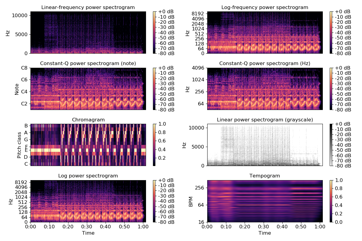
Visualize an STFT power spectrum

>>> import matplotlib.pyplot as plt
>>> y, sr = librosa.load(librosa.util.example_audio_file())
>>> plt.figure(figsize=(12, 8))

>>> D = librosa.amplitude_to_db(librosa.stft(y), ref=np.max)
>>> plt.subplot(4, 2, 1)
>>> librosa.display.specshow(D, y_axis='linear')
>>> plt.colorbar(format='%+2.0f dB')
>>> plt.title('Linear-frequency power spectrogram')

Or on a logarithmic scale

>>> plt.subplot(4, 2, 2)
>>> librosa.display.specshow(D, y_axis='log')
>>> plt.colorbar(format='%+2.0f dB')
>>> plt.title('Log-frequency power spectrogram')

Or use a CQT scale

>>> CQT = librosa.amplitude_to_db(librosa.cqt(y, sr=sr), ref=np.max)
>>> plt.subplot(4, 2, 3)
>>> librosa.display.specshow(CQT, y_axis='cqt_note')
>>> plt.colorbar(format='%+2.0f dB')
>>> plt.title('Constant-Q power spectrogram (note)')

>>> plt.subplot(4, 2, 4)
>>> librosa.display.specshow(CQT, y_axis='cqt_hz')
>>> plt.colorbar(format='%+2.0f dB')
>>> plt.title('Constant-Q power spectrogram (Hz)')

Draw a chromagram with pitch classes

>>> C = librosa.feature.chroma_cqt(y=y, sr=sr)
>>> plt.subplot(4, 2, 5)
>>> librosa.display.specshow(C, y_axis='chroma')
>>> plt.colorbar()
>>> plt.title('Chromagram')

Force a grayscale colormap (white -> black)

>>> plt.subplot(4, 2, 6)
>>> librosa.display.specshow(D, cmap='gray_r', y_axis='linear')
>>> plt.colorbar(format='%+2.0f dB')
>>> plt.title('Linear power spectrogram (grayscale)')

Draw time markers automatically

>>> plt.subplot(4, 2, 7)
>>> librosa.display.specshow(D, x_axis='time', y_axis='log')
>>> plt.colorbar(format='%+2.0f dB')
>>> plt.title('Log power spectrogram')

Draw a tempogram with BPM markers

>>> plt.subplot(4, 2, 8)
>>> Tgram = librosa.feature.tempogram(y=y, sr=sr)
>>> librosa.display.specshow(Tgram, x_axis='time', y_axis='tempo')
>>> plt.colorbar()
>>> plt.title('Tempogram')
>>> plt.tight_layout()

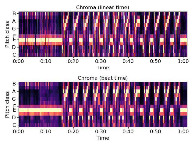
Draw beat-synchronous chroma in natural time

>>> plt.figure()
>>> tempo, beat_f = librosa.beat.beat_track(y=y, sr=sr, trim=False)
>>> beat_f = librosa.util.fix_frames(beat_f, x_max=C.shape[1])
>>> Csync = librosa.util.sync(C, beat_f, aggregate=np.median)
>>> beat_t = librosa.frames_to_time(beat_f, sr=sr)
>>> ax1 = plt.subplot(2,1,1)
>>> librosa.display.specshow(C, y_axis='chroma', x_axis='time')
>>> plt.title('Chroma (linear time)')
>>> ax2 = plt.subplot(2,1,2, sharex=ax1)
>>> librosa.display.specshow(Csync, y_axis='chroma', x_axis='time',
...                          x_coords=beat_t)
>>> plt.title('Chroma (beat time)')
>>> plt.tight_layout()

(Source code)