librosa.feature.tempogram

librosa.feature.tempogram(y=None, sr=22050, onset_envelope=None, hop_length=512, win_length=384, center=True, window=’hann’, norm=inf)

Compute the tempogram: local autocorrelation of the onset strength envelope. [1]

[1]	Grosche, Peter, Meinard Müller, and Frank Kurth. “Cyclic tempogram - A mid-level tempo representation for music signals.” ICASSP, 2010.

Parameters:

y : np.ndarray [shape=(n,)] or None

Audio time series.

sr : number > 0 [scalar]

sampling rate of y

onset_envelope : np.ndarray [shape=(n,) or (m, n)] or None

Optional pre-computed onset strength envelope as provided by onset.onset_strength.

If multi-dimensional, tempograms are computed independently for each band (first dimension).

hop_length : int > 0

number of audio samples between successive onset measurements

win_length : int > 0

length of the onset autocorrelation window (in frames/onset measurements) The default settings (384) corresponds to 384 * hop_length / sr ~= 8.9s.

center : bool

If True, onset autocorrelation windows are centered. If False, windows are left-aligned.

window : string, function, number, tuple, or np.ndarray [shape=(win_length,)]

A window specification as in core.stft.

norm : {np.inf, -np.inf, 0, float > 0, None}

Normalization mode. Set to None to disable normalization.

Returns:

tempogram : np.ndarray [shape=(win_length, n) or (m, win_length, n)]

Localized autocorrelation of the onset strength envelope.

If given multi-band input (onset_envelope.shape==(m,n)) then tempogram[i] is the tempogram of onset_envelope[i].

Raises:

ParameterError

if neither y nor onset_envelope are provided

if win_length < 1

See also

librosa.onset.onset_strength, librosa.util.normalize, librosa.core.stft

Examples

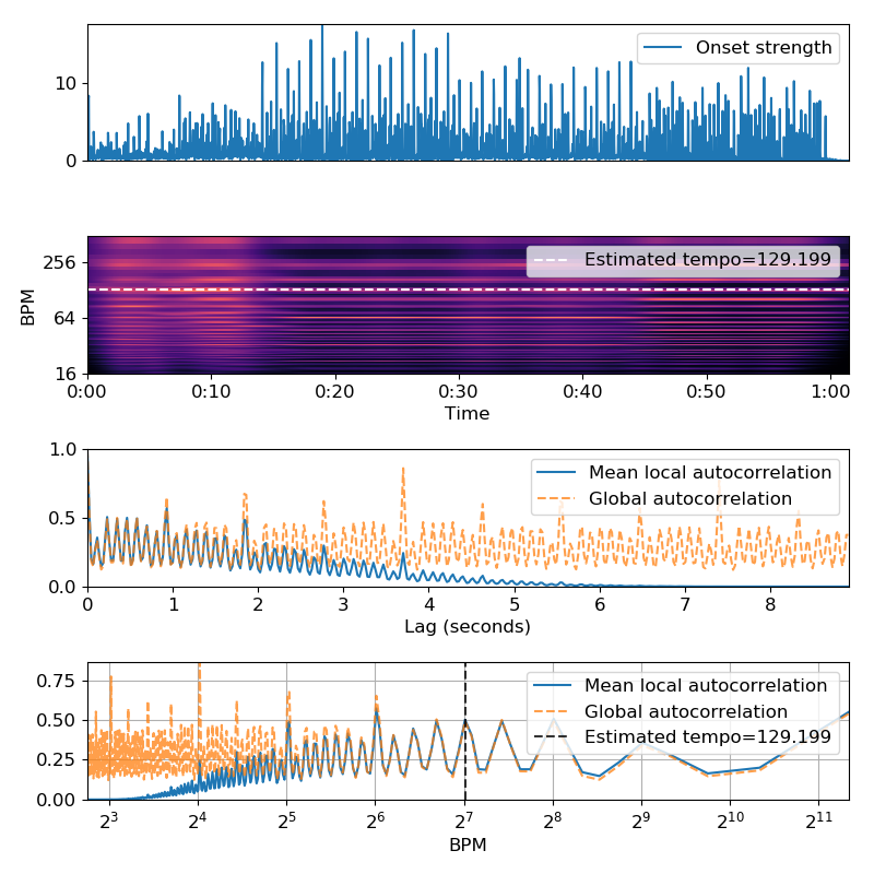
>>> # Compute local onset autocorrelation
>>> y, sr = librosa.load(librosa.util.example_audio_file())
>>> hop_length = 512
>>> oenv = librosa.onset.onset_strength(y=y, sr=sr, hop_length=hop_length)
>>> tempogram = librosa.feature.tempogram(onset_envelope=oenv, sr=sr,
...                                       hop_length=hop_length)
>>> # Compute global onset autocorrelation
>>> ac_global = librosa.autocorrelate(oenv, max_size=tempogram.shape[0])
>>> ac_global = librosa.util.normalize(ac_global)
>>> # Estimate the global tempo for display purposes
>>> tempo = librosa.beat.tempo(onset_envelope=oenv, sr=sr,
...                            hop_length=hop_length)[0]

>>> import matplotlib.pyplot as plt
>>> plt.figure(figsize=(8, 8))
>>> plt.subplot(4, 1, 1)
>>> plt.plot(oenv, label='Onset strength')
>>> plt.xticks([])
>>> plt.legend(frameon=True)
>>> plt.axis('tight')
>>> plt.subplot(4, 1, 2)
>>> # We'll truncate the display to a narrower range of tempi
>>> librosa.display.specshow(tempogram, sr=sr, hop_length=hop_length,
>>>                          x_axis='time', y_axis='tempo')
>>> plt.axhline(tempo, color='w', linestyle='--', alpha=1,
...             label='Estimated tempo={:g}'.format(tempo))
>>> plt.legend(frameon=True, framealpha=0.75)
>>> plt.subplot(4, 1, 3)
>>> x = np.linspace(0, tempogram.shape[0] * float(hop_length) / sr,
...                 num=tempogram.shape[0])
>>> plt.plot(x, np.mean(tempogram, axis=1), label='Mean local autocorrelation')
>>> plt.plot(x, ac_global, '--', alpha=0.75, label='Global autocorrelation')
>>> plt.xlabel('Lag (seconds)')
>>> plt.axis('tight')
>>> plt.legend(frameon=True)
>>> plt.subplot(4,1,4)
>>> # We can also plot on a BPM axis
>>> freqs = librosa.tempo_frequencies(tempogram.shape[0], hop_length=hop_length, sr=sr)
>>> plt.semilogx(freqs[1:], np.mean(tempogram[1:], axis=1),
...              label='Mean local autocorrelation', basex=2)
>>> plt.semilogx(freqs[1:], ac_global[1:], '--', alpha=0.75,
...              label='Global autocorrelation', basex=2)
>>> plt.axvline(tempo, color='black', linestyle='--', alpha=.8,
...             label='Estimated tempo={:g}'.format(tempo))
>>> plt.legend(frameon=True)
>>> plt.xlabel('BPM')
>>> plt.axis('tight')
>>> plt.grid()
>>> plt.tight_layout()

(Source code)