Derivatives in Theano
Computing Gradients
Now let’s use Theano for a slightly more sophisticated task: create a
function which computes the derivative of some expression y with
respect to its parameter x. To do this we will use the macro T.grad.
For instance, we can compute the
gradient of  with respect to
  . Note that:
 .
.
Here is the code to compute this gradient:
>>> import theano
>>> import theano.tensor as T
>>> from theano import pp
>>> x = T.dscalar('x')
>>> y = x ** 2
>>> gy = T.grad(y, x)
>>> pp(gy)  # print out the gradient prior to optimization
'((fill((x ** TensorConstant{2}), TensorConstant{1.0}) * TensorConstant{2}) * (x ** (TensorConstant{2} - TensorConstant{1})))'
>>> f = theano.function([x], gy)
>>> f(4)
array(8.0)
>>> f(94.2)
array(188.4)
In this example, we can see from pp(gy) that we are computing
the correct symbolic gradient.
fill((x ** 2), 1.0) means to make a matrix of the same shape as
x ** 2 and fill it with 1.0.
Note
The optimizer simplifies the symbolic gradient expression. You can see this by digging inside the internal properties of the compiled function.
pp(f.maker.fgraph.outputs[0])
'(2.0 * x)'
After optimization there is only one Apply node left in the graph, which doubles the input.
We can also compute the gradient of complex expressions such as the
logistic function defined above. It turns out that the derivative of the
logistic is:  .
.
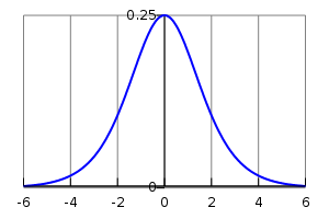
A plot of the gradient of the logistic function, with x on the x-axis
and  on the y-axis.
>>> x = T.dmatrix('x')
>>> s = T.sum(1 / (1 + T.exp(-x)))
>>> gs = T.grad(s, x)
>>> dlogistic = theano.function([x], gs)
>>> dlogistic([[0, 1], [-1, -2]])
array([[ 0.25      ,  0.19661193],
       [ 0.19661193,  0.10499359]])
In general, for any scalar expression s, T.grad(s, w) provides
the Theano expression for computing  . In
this way Theano can be used for doing efficient symbolic differentiation
(as the expression returned by
. In
this way Theano can be used for doing efficient symbolic differentiation
(as the expression returned by T.grad will be optimized during compilation), even for
function with many inputs. (see automatic differentiation for a description
of symbolic differentiation).
Note
The second argument of T.grad can be a list, in which case the
output is also a list. The order in both lists is important: element
i of the output list is the gradient of the first argument of
T.grad with respect to the i-th element of the list given as second argument.
The first argument of T.grad has to be a scalar (a tensor
of size 1). For more information on the semantics of the arguments of
T.grad and details about the implementation, see
this section of the library.
Additional information on the inner workings of differentiation may also be found in the more advanced tutorial Extending Theano.
Computing the Jacobian
In Theano’s parlance, the term Jacobian designates the tensor comprising the
first partial derivatives of the output of a function with respect to its inputs.
(This is a generalization of to the so-called Jacobian matrix in Mathematics.)
Theano implements the theano.gradient.jacobian() macro that does all
that is needed to compute the Jacobian. The following text explains how
to do it manually.
In order to manually compute the Jacobian of some function y with
respect to some parameter x we need to use scan. What we
do is to loop over the entries in y and compute the gradient of
y[i] with respect to x.
Note
scan is a generic op in Theano that allows writing in a symbolic
manner all kinds of recurrent equations. While creating
symbolic loops (and optimizing them for performance) is a hard task,
effort is being done for improving the performance of scan. We
shall return to scan later in this tutorial.
>>> import theano
>>> import theano.tensor as T
>>> x = T.dvector('x')
>>> y = x ** 2
>>> J, updates = theano.scan(lambda i, y,x : T.grad(y[i], x), sequences=T.arange(y.shape[0]), non_sequences=[y,x])
>>> f = theano.function([x], J, updates=updates)
>>> f([4, 4])
array([[ 8.,  0.],
       [ 0.,  8.]])
What we do in this code is to generate a sequence of ints from 0 to
y.shape[0] using T.arange. Then we loop through this sequence, and
at each step, we compute the gradient of element y[i] with respect to
x. scan automatically concatenates all these rows, generating a
matrix which corresponds to the Jacobian.
Note
There are some pitfalls to be aware of regarding T.grad. One of them is that you
cannot re-write the above expression of the Jacobian as
theano.scan(lambda y_i,x: T.grad(y_i,x), sequences=y,
non_sequences=x)
, even though from the documentation of scan this
seems possible. The reason is that y_i will not be a function of
x anymore, while y[i] still is.
Computing the Hessian
In Theano, the term Hessian has the usual mathematical acception: It is the
matrix comprising the second order partial derivative of a function with scalar
output and vector input. Theano implements theano.gradient.hessian() macro that does all
that is needed to compute the Hessian. The following text explains how
to do it manually.
You can compute the Hessian manually similarly to the Jacobian. The only
difference is that now, instead of computing the Jacobian of some expression
y, we compute the Jacobian of T.grad(cost,x), where cost is some
scalar.
>>> x = T.dvector('x')
>>> y = x ** 2
>>> cost = y.sum()
>>> gy = T.grad(cost, x)
>>> H, updates = theano.scan(lambda i, gy,x : T.grad(gy[i], x), sequences=T.arange(gy.shape[0]), non_sequences=[gy, x])
>>> f = theano.function([x], H, updates=updates)
>>> f([4, 4])
array([[ 2.,  0.],
       [ 0.,  2.]])
Jacobian times a Vector
Sometimes we can express the algorithm in terms of Jacobians times vectors, or vectors times Jacobians. Compared to evaluating the Jacobian and then doing the product, there are methods that compute the desired results while avoiding actual evaluation of the Jacobian. This can bring about significant performance gains. A description of one such algorithm can be found here:
- Barak A. Pearlmutter, “Fast Exact Multiplication by the Hessian”, Neural Computation, 1994
While in principle we would want Theano to identify these patterns automatically for us, in practice, implementing such optimizations in a generic manner is extremely difficult. Therefore, we provide special functions dedicated to these tasks.
R-operator
The R operator is built to evaluate the product between a Jacobian and a
vector, namely  . The formulation
can be extended even for x being a matrix, or a tensor in general, case in
which also the Jacobian becomes a tensor and the product becomes some kind
of tensor product. Because in practice we end up needing to compute such
expressions in terms of weight matrices, Theano supports this more generic
form of the operation. In order to evaluate the R-operation of
expression y, with respect to x, multiplying the Jacobian with v
you need to do something similar to this:
. The formulation
can be extended even for x being a matrix, or a tensor in general, case in
which also the Jacobian becomes a tensor and the product becomes some kind
of tensor product. Because in practice we end up needing to compute such
expressions in terms of weight matrices, Theano supports this more generic
form of the operation. In order to evaluate the R-operation of
expression y, with respect to x, multiplying the Jacobian with v
you need to do something similar to this:
>>> W = T.dmatrix('W')
>>> V = T.dmatrix('V')
>>> x = T.dvector('x')
>>> y = T.dot(x, W)
>>> JV = T.Rop(y, W, V)
>>> f = theano.function([W, V, x], JV)
>>> f([[1, 1], [1, 1]], [[2, 2], [2, 2]], [0,1])
array([ 2.,  2.])
List of Op that implement Rop.
L-operator
In similitude to the R-operator, the L-operator would compute a row vector times
the Jacobian. The mathematical formula would be  . The L-operator is also supported for generic tensors
(not only for vectors). Similarly, it can be implemented as follows:
. The L-operator is also supported for generic tensors
(not only for vectors). Similarly, it can be implemented as follows:
>>> W = T.dmatrix('W')
>>> v = T.dvector('v')
>>> x = T.dvector('x')
>>> y = T.dot(x, W)
>>> VJ = T.Lop(y, W, v)
>>> f = theano.function([v,x], VJ)
>>> f([2, 2], [0, 1])
array([[ 0.,  0.],
       [ 2.,  2.]])
Note
v, the point of evaluation, differs between the L-operator and the R-operator. For the L-operator, the point of evaluation needs to have the same shape as the output, whereas for the R-operator this point should have the same shape as the input parameter. Furthermore, the results of these two operations differ. The result of the L-operator is of the same shape as the input parameter, while the result of the R-operator has a shape similar to that of the output.
Hessian times a Vector
If you need to compute the Hessian times a vector, you can make use of the above-defined operators to do it more efficiently than actually computing the exact Hessian and then performing the product. Due to the symmetry of the Hessian matrix, you have two options that will give you the same result, though these options might exhibit differing performances. Hence, we suggest profiling the methods before using either one of the two:
>>> x = T.dvector('x')
>>> v = T.dvector('v')
>>> y = T.sum(x ** 2)
>>> gy = T.grad(y, x)
>>> vH = T.grad(T.sum(gy * v), x)
>>> f = theano.function([x, v], vH)
>>> f([4, 4], [2, 2])
array([ 4.,  4.])
or, making use of the R-operator:
>>> x = T.dvector('x')
>>> v = T.dvector('v')
>>> y = T.sum(x ** 2)
>>> gy = T.grad(y, x)
>>> Hv = T.Rop(gy, x, v)
>>> f = theano.function([x, v], Hv)
>>> f([4, 4], [2, 2])
array([ 4.,  4.])
Final Pointers
- The
gradfunction works symbolically: it receives and returns Theano variables. gradcan be compared to a macro since it can be applied repeatedly.- Scalar costs only can be directly handled by
grad. Arrays are handled through repeated applications. - Built-in functions allow to compute efficiently vector times Jacobian and vector times Hessian.
- Work is in progress on the optimizations required to compute efficiently the full Jacobian and the Hessian matrix as well as the Jacobian times vector.