What is CVXPY?¶

CVXPY is a Python-embedded modeling language for convex optimization problems. It automatically transforms the problem into standard form, calls a solver, and unpacks the results.

The code below solves a simple optimization problem in CVXPY:

from cvxpy import *

# Create two scalar optimization variables.
x = Variable()
y = Variable()

# Create two constraints.
constraints = [x + y == 1,
               x - y >= 1]

# Form objective.
obj = Minimize(square(x - y))

# Form and solve problem.
prob = Problem(obj, constraints)
prob.solve()  # Returns the optimal value.
print "status:", prob.status
print "optimal value", prob.value
print "optimal var", x.value, y.value

status: optimal
optimal value 0.999999999761
optimal var 1.00000000001 -1.19961841702e-11

The status, which was assigned a value “optimal” by the solve method, tells us the problem was solved successfully. The optimal value (basically 1 here) is the minimum value of the objective over all choices of variables that satisfy the constraints. The last thing printed gives values of x and y (basically 1 and 0 respectively) that achieve the optimal objective.

prob.solve() returns the optimal value and updates prob.status, prob.value, and the value field of all the variables in the problem.

Namespace¶

The Python examples in this tutorial import CVXPY using the syntax from cvxpy import *. This is done to make the examples simpler and more concise. But for production code you should always import CVXPY as a namespace. For example, import cvxpy as cvx. Here’s the code from the previous section with CVXPY imported as a namespace.

import cvxpy as cvx

# Create two scalar optimization variables.
x = cvx.Variable()
y = cvx.Variable()

# Create two constraints.
constraints = [x + y == 1,
               x - y >= 1]

# Form objective.
obj = cvx.Minimize(cvx.square(x - y))

# Form and solve problem.
prob = cvx.Problem(obj, constraints)
prob.solve()  # Returns the optimal value.
print "status:", prob.status
print "optimal value", prob.value
print "optimal var", x.value, y.value

Nonetheless we have designed CVXPY so that using from cvxpy import * is generally safe for short scripts. The biggest catch is that the built-in max and min cannot be used on CVXPY expressions. Instead use the CVXPY functions max_elemwise, max_entries, min_elemwise, or min_entries.

The built-in sum can be used on lists of CVXPY expressions to add all the list elements together. Use the CVXPY function sum_entries to sum the entries of a single CVXPY matrix or vector expression.

Changing the problem¶

After you create a problem object, you can still modify the objective and constraints.

# Replace the objective.
prob.objective = Maximize(x + y)
print "optimal value", prob.solve()

# Replace the constraint (x + y == 1).
prob.constraints[0] = (x + y <= 3)
print "optimal value", prob.solve()

optimal value 1.0
optimal value 3.00000000006

Infeasible and unbounded problems¶

If a problem is infeasible or unbounded, the status field will be set to “infeasible” or “unbounded”, respectively. The value fields of the problem variables are not updated.

from cvxpy import *

x = Variable()

# An infeasible problem.
prob = Problem(Minimize(x), [x >= 1, x <= 0])
prob.solve()
print "status:", prob.status
print "optimal value", prob.value

# An unbounded problem.
prob = Problem(Minimize(x))
prob.solve()
print "status:", prob.status
print "optimal value", prob.value

status: infeasible
optimal value inf
status: unbounded
optimal value -inf

Notice that for a minimization problem the optimal value is inf if infeasible and -inf if unbounded. For maximization problems the opposite is true.

Vectors and matrices¶

Variables can be scalars, vectors, or matrices.

# A scalar variable.
a = Variable()

# Column vector variable of length 5.
x = Variable(5)

# Matrix variable with 4 rows and 7 columns.
A = Variable(4, 7)

You can use your numeric library of choice to construct matrix and vector constants. For instance, if x is a CVXPY Variable in the expression A*x + b, A and b could be Numpy ndarrays, SciPy sparse matrices, etc. A and b could even be different types.

Currently the following types may be used as constants:

Numpy ndarrays
Numpy matrices
SciPy sparse matrices

Here’s an example of a CVXPY problem with vectors and matrices:

# Solves a bounded least-squares problem.

from cvxpy import *
import numpy

# Problem data.
m = 10
n = 5
numpy.random.seed(1)
A = numpy.random.randn(m, n)
b = numpy.random.randn(m, 1)

# Construct the problem.
x = Variable(n)
objective = Minimize(sum_entries(square(A*x - b)))
constraints = [0 <= x, x <= 1]
prob = Problem(objective, constraints)

print "Optimal value", prob.solve()
print "Optimal var"
print x.value # A numpy matrix.

Optimal value 4.14133859146
Optimal var
[[ -2.76479783e-10]
 [  3.59742090e-10]
 [  1.34633378e-01]
 [  1.24978611e-01]
 [ -3.67846924e-11]]

Constraints¶

As shown in the example code, you can use ==, <=, and >= to construct constraints in CVXPY. Equality and inequality constraints are elementwise, whether they involve scalars, vectors, or matrices. For example, together the constraints 0 <= x and x <= 1 mean that every entry of x is between 0 and 1.

If you want matrix inequalities that represent semi-definite cone constraints, see Semidefinite matrices. The section explains how to express a semi-definite cone inequality.

You cannot construct inequalities with < and >. Strict inequalities don’t make sense in a real world setting. Also, you cannot chain constraints together, e.g., 0 <= x <= 1 or x == y == 2. The Python interpreter treats chained constraints in such a way that CVXPY cannot capture them. CVXPY will raise an exception if you write a chained constraint.

Parameters¶

Parameters are symbolic representations of constants. The purpose of parameters is to change the value of a constant in a problem without reconstructing the entire problem.

Parameters can be vectors or matrices, just like variables. When you create a parameter you have the option of specifying the sign of the parameter’s entries (positive, negative, or unknown). The sign is unknown by default. The sign is used in Disciplined Convex Programming. Parameters can be assigned a constant value any time after they are created. The constant value must have the same dimensions and sign as those specified when the parameter was created.

# Positive scalar parameter.
m = Parameter(sign="positive")

# Column vector parameter with unknown sign (by default).
c = Parameter(5)

# Matrix parameter with negative entries.
G = Parameter(4, 7, sign="negative")

# Assigns a constant value to G.
G.value = -numpy.ones((4, 7))

You can initialize a parameter with a value. The following code segments are equivalent:

# Create parameter, then assign value.
rho = Parameter(sign="positive")
rho.value = 2

# Initialize parameter with a value.
rho = Parameter(sign="positive", value=2)

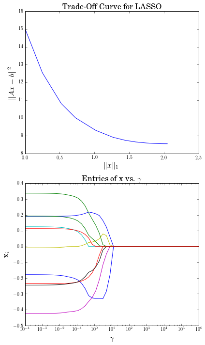
Computing trade-off curves is a common use of parameters. The example below computes a trade-off curve for a LASSO problem.

from cvxpy import *
import numpy
import matplotlib.pyplot as plt

# Problem data.
n = 15
m = 10
numpy.random.seed(1)
A = numpy.random.randn(n, m)
b = numpy.random.randn(n, 1)
# gamma must be positive due to DCP rules.
gamma = Parameter(sign="positive")

# Construct the problem.
x = Variable(m)
error = sum_squares(A*x - b)
obj = Minimize(error + gamma*norm(x, 1))
prob = Problem(obj)

# Construct a trade-off curve of ||Ax-b||^2 vs. ||x||_1
sq_penalty = []
l1_penalty = []
x_values = []
gamma_vals = numpy.logspace(-4, 6)
for val in gamma_vals:
    gamma.value = val
    prob.solve()
    # Use expr.value to get the numerical value of
    # an expression in the problem.
    sq_penalty.append(error.value)
    l1_penalty.append(norm(x, 1).value)
    x_values.append(x.value)

plt.rc('text', usetex=True)
plt.rc('font', family='serif')
plt.figure(figsize=(6,10))

# Plot trade-off curve.
plt.subplot(211)
plt.plot(l1_penalty, sq_penalty)
plt.xlabel(r'\|x\|_1', fontsize=16)
plt.ylabel(r'\|Ax-b\|^2', fontsize=16)
plt.title('Trade-Off Curve for LASSO', fontsize=16)

# Plot entries of x vs. gamma.
plt.subplot(212)
for i in range(m):
    plt.plot(gamma_vals, [xi[i,0] for xi in x_values])
plt.xlabel(r'\gamma', fontsize=16)
plt.ylabel(r'x_{i}', fontsize=16)
plt.xscale('log')
plt.title(r'\text{Entries of x vs. }\gamma', fontsize=16)

plt.tight_layout()
plt.show()

Trade-off curves can easily be computed in parallel. The code below computes in parallel the optimal x for each \(\gamma\) in the LASSO problem above.

from multiprocessing import Pool

# Assign a value to gamma and find the optimal x.
def get_x(gamma_value):
    gamma.value = gamma_value
    result = prob.solve()
    return x.value

# Parallel computation (set to 1 process here).
pool = Pool(processes = 1)
x_values = pool.map(get_x, gamma_vals)