DCGAN: Generate images with Deep Convolutional GAN
0. Introduction
In this tutorial, we generate images with generative adversarial networks (GAN). GAN are kinds of deep neural network for generative modeling that are often applied to image generation. GAN-based models are also used in PaintsChainer, an automatic colorization service.
In this tutorial, you will learn the following things:
Generative Adversarial Networks (GAN)
Implementation of DCGAN in Chainer
1. Generarive Adversarial Networks (GAN)
1.1 What are GAN?
As explained in GAN tutorial in NIPS 2016 [1], generative models can be classified into the categories as shown in the following figure:
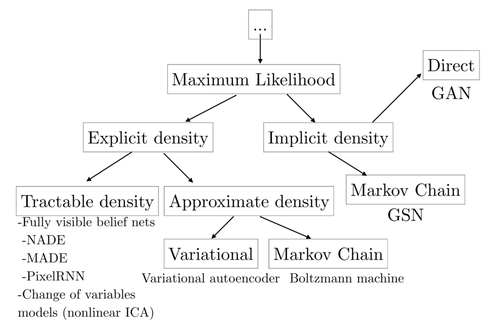
cited from [1]
Besides GAN, other famous generative models include Fully visible belief networks (FVBNs) and Variational autoencoder (VAE). Unlike FVBNs and VAE, GAN do not explicitly model the probability distribution \(p({\bf s})\) that generates training data. Instead, we model a generator \(G: {\bf z} \mapsto {\bf s}\). The generator \(G\) samples \({\bf s} \sim p({\bf s})\) from the latent variable \({\bf z}\). Apart from the generator \(G\), we create a discriminator \(D({\bf x})\) which discriminates between samples from the generator G and examples from training data. While training the discriminator \(D\), the generator \(G\) tries to maximize the probability of the discriminator \(D\) making a mistake. So, the generator \(G\) tries to create samples that seem to be drawn from the same distribution as the training data.
The advantages of GAN are low sampling cost and its state-of-the-art performance in image generation. The disadvantage is that we cannot calculate the likelihood \(p_{\mathrm {model}}({\bf s})\) because we do not model any probability distribution, and we cannot infer the latent variable \({\bf z}\) from a sample.
1.2 How GAN work?
As explained above, GAN use the two models, the generator and the discriminator. When training the networks, we should match the data distribution \(p({\bf s})\) with the distribution of the samples \({\bf s} = G ({\bf z})\) generated from the generator.
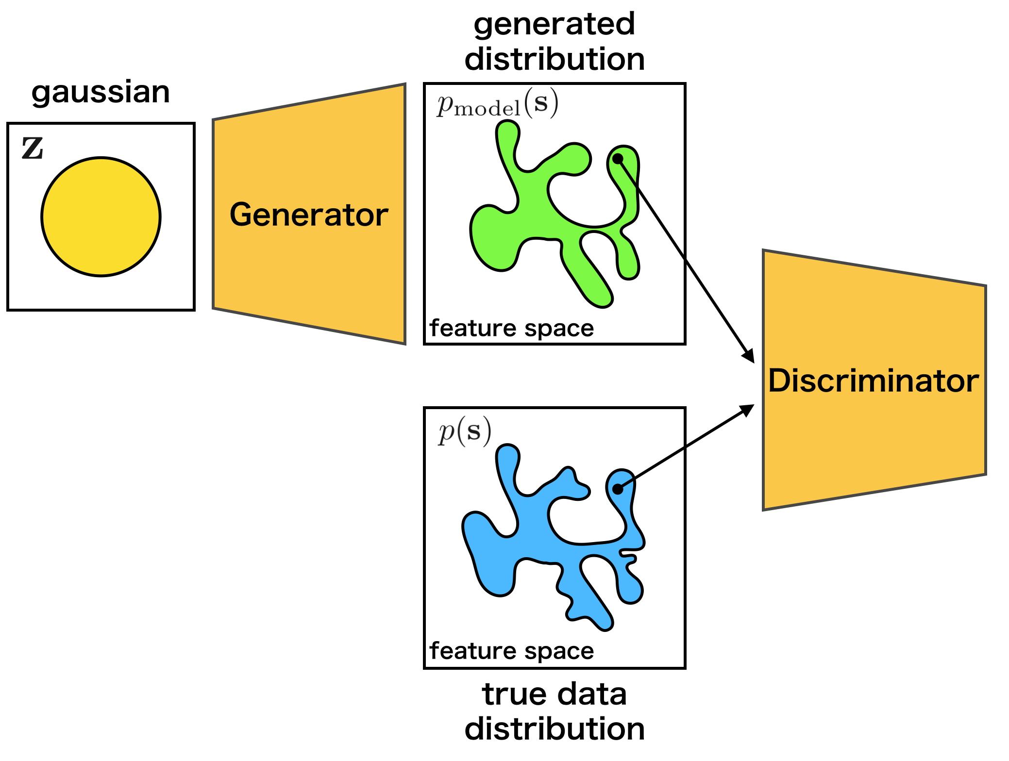
The generator \(G\) learns the target distribution, and ideally eventually reaches a Nash equilibrium [2] of game theory. In detail, while training the discriminator \(D\), the generator \(G\) is also trained, so that the discriminator \(D\) makes a mistake.
As an intuitive example, the relationship between counterfeiters of banknotes and the police is frequently used. The counterfeiters try to make counterfeit notes that look like real banknotes. The police try to distinguish real bank notes from counterfeit notes. It is supposed that the ability of the police gradually rises, so that real banknotes and counterfeit notes can be recognized well. Then, the counterfeiters will not be able to use counterfeit banknotes, so they will create counterfeit banknotes that appear more realistic. As the police improve their skill further, they can distinguish real and counterfeit notes… Eventually, the counterfeiter will be able to produce counterfeit banknotes look as real as genuine ones.
The training process is explained by the following mathematical expressions. First, since the discriminator \(D({\bf s})\) is the probability that a sample \({\bf s}\) is generated from the data distribution at, it can be expressed as follows:
Then, when we match the data distribution \({\bf s} \sim p({\bf s})\) and the distribution of generated samples by \(G\), it means that we should minimize the dissimilarity between the two distributions. It is common to use Jensen-Shannon Divergence \(D_{\mathrm{JS}}\) to measure the dissimilarity between distributions[3].
The \(D_{\mathrm{JS}}\) of \(p_{\mathrm{model}}({\bf s})\) and \(p({\bf s})\) can be written as follows by using \(D({\bf s})\):
where \(\bar{p}({\bf s}) = \frac{p({\bf s}) + p_{\rm model}({\bf s})}{2}\). The \(D_{\mathrm{JS}}\) will be ma{bf s}imized by the discriminator \(D\) and minimized by the generator \(G\), namely, \(p_{\mathrm{model}}\). And the distribution \(p_{\mathrm model}({\bf s})\) generated by \(G({\bf {\bf s}})\) can match the data distribution \(p({\bf s})\).
When we actually train the model, the above min-max problem is solved by alternately updating the discriminator \(D({\bf s})\) and the generator \(G({\bf z})\) [4]. The actual training procedures are described as follows:
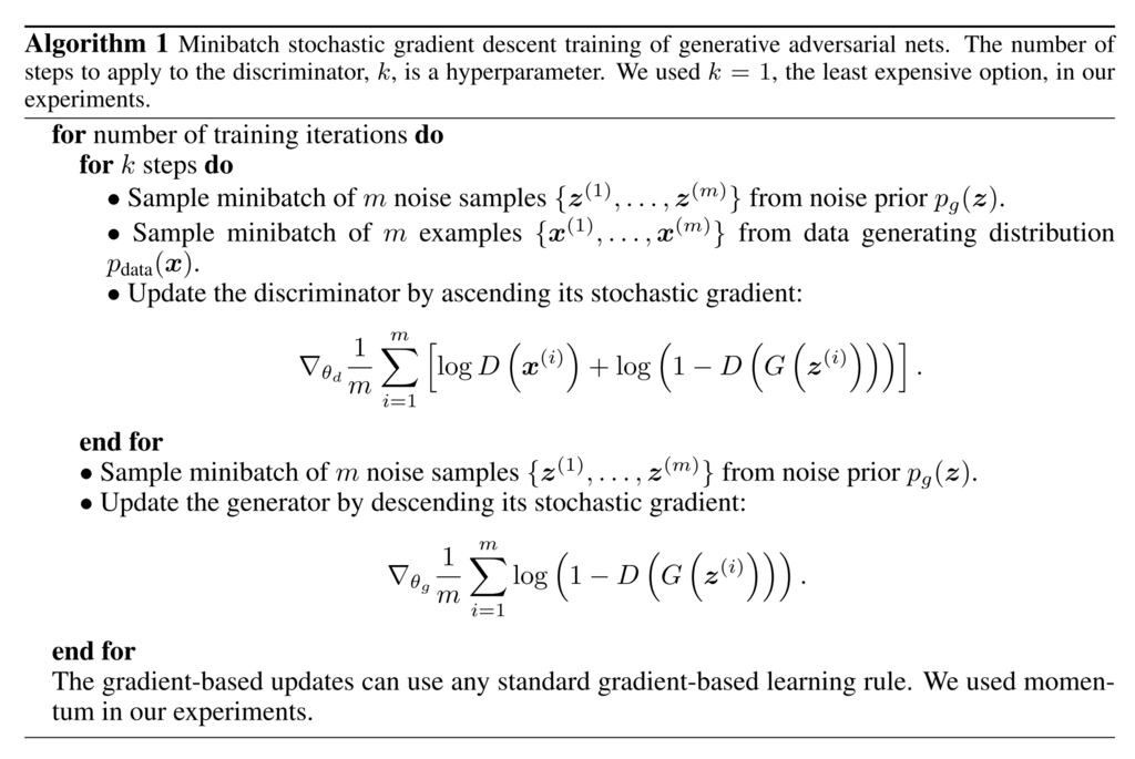
cited from [4]
1.3 What are DCGAN?
In this section, we will introduce the model called DCGAN(Deep Convolutional GAN) proposed by Radford et al.[5]. As shown below, it is a model using CNN(Convolutional Neural Network) as its name suggests.

cited from [5]
In addition, although GAN are known for its difficulty in training, this paper introduces various techniques for successful training:
Convert max-pooling layers to convolution layers with larger or fractional strides
Convert fully connected layers to global average pooling layers in the discriminator
Use batch normalization layers in the generator and the discriminator
Use leaky ReLU activation functions in the discriminator
2. Implementation of DCGAN in Chainer
There is an example of DCGAN in the official repository of Chainer, so we will explain how to implement DCGAN based on this: chainer/examples/dcgan
2.1 Define the generator model
First, let’s define a network for the generator.
class Generator(chainer.Chain):

    def __init__(self, n_hidden, bottom_width=4, ch=512, wscale=0.02):
        super(Generator, self).__init__()
        self.n_hidden = n_hidden
        self.ch = ch
        self.bottom_width = bottom_width

        with self.init_scope():
            w = chainer.initializers.Normal(wscale)
            self.l0 = L.Linear(self.n_hidden, bottom_width * bottom_width * ch,
                               initialW=w)
            self.dc1 = L.Deconvolution2D(ch, ch // 2, 4, 2, 1, initialW=w)
            self.dc2 = L.Deconvolution2D(ch // 2, ch // 4, 4, 2, 1, initialW=w)
            self.dc3 = L.Deconvolution2D(ch // 4, ch // 8, 4, 2, 1, initialW=w)
            self.dc4 = L.Deconvolution2D(ch // 8, 3, 3, 1, 1, initialW=w)
            self.bn0 = L.BatchNormalization(bottom_width * bottom_width * ch)
            self.bn1 = L.BatchNormalization(ch // 2)
            self.bn2 = L.BatchNormalization(ch // 4)
            self.bn3 = L.BatchNormalization(ch // 8)

    def make_hidden(self, batchsize):
        dtype = chainer.get_dtype()
        return numpy.random.uniform(-1, 1, (batchsize, self.n_hidden, 1, 1))\
            .astype(dtype)

    def forward(self, z):
        h = F.reshape(F.relu(self.bn0(self.l0(z))),
                      (len(z), self.ch, self.bottom_width, self.bottom_width))
        h = F.relu(self.bn1(self.dc1(h)))
        h = F.relu(self.bn2(self.dc2(h)))
        h = F.relu(self.bn3(self.dc3(h)))
        x = F.sigmoid(self.dc4(h))
        return x
When we make a network in Chainer, there are some conventions:
Define a network class which inherits
Chain.Make
chainer.links’s instances in theinit_scope():of the initializer__init__.Define network connections in the
__call__operator by using thechainer.links’s instances andchainer.functions.
If you are not familiar with constructing a new network, please refer to this tutorial.
As we can see from the initializer __init__, the Generator
uses deconvolution layers Deconvolution2D
and batch normalization layers BatchNormalization.
In __call__, each layer is called and followed by
relu except the last layer.
Because the first argument of L.Deconvolution is the channel size of input and
the second is the channel size of output, we can find that each layer halves the
channel size. When we construct Generator with ch=1024, the network
is same as the above image.
Note
Be careful when passing the output of a fully connected layer to a convolution
layer, because the convolutional layer needs additional dimensions for inputs.
As we can see the 1st line of __call__,
the output of the fully connected layer is reshaped by reshape
to add the dimensions of the channel, the width and the height of images.
2.2 Define the discriminator model
In addtion, let’s define the network for the discriminator.
class Discriminator(chainer.Chain):

    def __init__(self, bottom_width=4, ch=512, wscale=0.02):
        w = chainer.initializers.Normal(wscale)
        super(Discriminator, self).__init__()
        with self.init_scope():
            self.c0_0 = L.Convolution2D(3, ch // 8, 3, 1, 1, initialW=w)
            self.c0_1 = L.Convolution2D(ch // 8, ch // 4, 4, 2, 1, initialW=w)
            self.c1_0 = L.Convolution2D(ch // 4, ch // 4, 3, 1, 1, initialW=w)
            self.c1_1 = L.Convolution2D(ch // 4, ch // 2, 4, 2, 1, initialW=w)
            self.c2_0 = L.Convolution2D(ch // 2, ch // 2, 3, 1, 1, initialW=w)
            self.c2_1 = L.Convolution2D(ch // 2, ch // 1, 4, 2, 1, initialW=w)
            self.c3_0 = L.Convolution2D(ch // 1, ch // 1, 3, 1, 1, initialW=w)
            self.l4 = L.Linear(bottom_width * bottom_width * ch, 1, initialW=w)
            self.bn0_1 = L.BatchNormalization(ch // 4, use_gamma=False)
            self.bn1_0 = L.BatchNormalization(ch // 4, use_gamma=False)
            self.bn1_1 = L.BatchNormalization(ch // 2, use_gamma=False)
            self.bn2_0 = L.BatchNormalization(ch // 2, use_gamma=False)
            self.bn2_1 = L.BatchNormalization(ch // 1, use_gamma=False)
            self.bn3_0 = L.BatchNormalization(ch // 1, use_gamma=False)

    def forward(self, x):
        h = add_noise(x)
        h = F.leaky_relu(add_noise(self.c0_0(h)))
        h = F.leaky_relu(add_noise(self.bn0_1(self.c0_1(h))))
        h = F.leaky_relu(add_noise(self.bn1_0(self.c1_0(h))))
        h = F.leaky_relu(add_noise(self.bn1_1(self.c1_1(h))))
        h = F.leaky_relu(add_noise(self.bn2_0(self.c2_0(h))))
        h = F.leaky_relu(add_noise(self.bn2_1(self.c2_1(h))))
        h = F.leaky_relu(add_noise(self.bn3_0(self.c3_0(h))))
        return self.l4(h)
The Discriminator network is almost mirrors of the Generator network.
However, there are minor different points:
Use
leaky_reluas activation functionsDeeper than
GeneratorAdd some noise to every intermediate outputs before giving them to the next layers
def add_noise(h, sigma=0.2):
    xp = backend.get_array_module(h.data)
    if chainer.config.train:
        return h + sigma * xp.random.randn(*h.shape)
    else:
        return h
2.3 Prepare dataset and iterator
Let’s retrieve the CIFAR-10 dataset by using Chainer’s dataset utility function
get_cifar10. CIFAR-10 is a set of small natural images.
Each example is an RGB color image of size 32x32. In the original images,
each of R, G, B of pixels is represented by one-byte unsigned integer
(i.e. from 0 to 255).
This function changes the scale of pixel values into [0, scale] float values.
train, _ = chainer.datasets.get_cifar10(withlabel=False, scale=255.)
train_iter = chainer.iterators.SerialIterator(train, args.batchsize)
2.4 Prepare model and optimizer
Let’s make the instances of the generator and the discriminator.
gen = Generator(n_hidden=args.n_hidden)
dis = Discriminator()
Next, let’s make optimizers for the models created above.
def make_optimizer(model, alpha=0.0002, beta1=0.5):
    optimizer = chainer.optimizers.Adam(alpha=alpha, beta1=beta1)
    optimizer.setup(model)
    optimizer.add_hook(
        chainer.optimizer_hooks.WeightDecay(0.0001), 'hook_dec')
    return optimizer

opt_gen = make_optimizer(gen)
opt_dis = make_optimizer(dis)
2.5 Prepare updater
GAN need the two models: the generator and the discriminator. Usually, the default updaters pre-defined in Chainer take only one model. So, we need to define a custom updater for GAN training.
The definition of DCGANUpdater is a little complicated. However, it just
minimizes the loss of the discriminator and that of the generator alternately.
As you can see in the class definiton, DCGANUpdater inherits
StandardUpdater. In this case,
almost all necessary functions are defined in
StandardUpdater,
we just override the functions of __init__ and update_core.
Note
We do not need to define loss_dis and loss_gen because the functions
are called only in update_core. It aims at improving readability.
class DCGANUpdater(chainer.training.updaters.StandardUpdater):

    def __init__(self, *args, **kwargs):
        self.gen, self.dis = kwargs.pop('models')
        super(DCGANUpdater, self).__init__(*args, **kwargs)

    def loss_dis(self, dis, y_fake, y_real):
        batchsize = len(y_fake)
        L1 = F.sum(F.softplus(-y_real)) / batchsize
        L2 = F.sum(F.softplus(y_fake)) / batchsize
        loss = L1 + L2
        chainer.report({'loss': loss}, dis)
        return loss

    def loss_gen(self, gen, y_fake):
        batchsize = len(y_fake)
        loss = F.sum(F.softplus(-y_fake)) / batchsize
        chainer.report({'loss': loss}, gen)
        return loss

    def update_core(self):
        gen_optimizer = self.get_optimizer('gen')
        dis_optimizer = self.get_optimizer('dis')

        batch = self.get_iterator('main').next()
        x_real = Variable(self.converter(batch, self.device)) / 255.
        xp = chainer.backend.get_array_module(x_real.data)

        gen, dis = self.gen, self.dis
        batchsize = len(batch)

        y_real = dis(x_real)

        z = Variable(xp.asarray(gen.make_hidden(batchsize)))
        x_fake = gen(z)
        y_fake = dis(x_fake)

        dis_optimizer.update(self.loss_dis, dis, y_fake, y_real)
        gen_optimizer.update(self.loss_gen, gen, y_fake)
In the intializer __init__, an addtional keyword argument models is
required as you can see the code below. Also, we use keyword arguments
iterator, optimizer and device.
It should be noted that the optimizer augment takes a dictionary.
The two different models require two different optimizers.
To specify the different optimizers for the models, we give a dictionary,
{'gen': opt_gen, 'dis': opt_dis}, to the optimizer argument.
we should input
optimizer as a dictionary {'gen': opt_gen, 'dis': opt_dis}.
In the DCGANUpdater, you can access the iterator with self.get_iterator('main').
Also, you can access the optimizers with
self.get_optimizer('gen') and self.get_optimizer('dis').
In update_core, the two loss functions loss_dis and loss_gen
are minimized by the optimizers. At first two lines, we access
the optimizers. Then, we create next minibatch of training data by
self.get_iterator('main').next(), copy batch to the device
by self.converter, and make it a Variable object.
After that, we minimize the loss functions with
the optimizers.
Note
When defining update_core, we may want to manipulate the
underlying array of a Variable with numpy or cupy library.
Note that the type of arrays on CPU is numpy.ndarray, while the type
of arrays on GPU is cupy.ndarray. However, users do not need to write
if condition explicitly, because the appropriate array module can be
obtained by xp = chainer.backends.cuda.get_array_module(variable.array).
If variable is on GPU, cupy is assigned to xp, otherwise
numpy is assigned to xp.
updater = DCGANUpdater(
    models=(gen, dis),
    iterator=train_iter,
    optimizer={
        'gen': opt_gen, 'dis': opt_dis},
    device=args.gpu)
2.6 Prepare trainer and run
trainer = training.Trainer(updater, (args.epoch, 'epoch'), out=args.out)

snapshot_interval = (args.snapshot_interval, 'iteration')
display_interval = (args.display_interval, 'iteration')
trainer.extend(
    extensions.snapshot(filename='snapshot_iter_{.updater.iteration}.npz'),
    trigger=snapshot_interval)
trainer.extend(extensions.snapshot_object(
    gen, 'gen_iter_{.updater.iteration}.npz'), trigger=snapshot_interval)
trainer.extend(extensions.snapshot_object(
    dis, 'dis_iter_{.updater.iteration}.npz'), trigger=snapshot_interval)
trainer.extend(extensions.LogReport(trigger=display_interval))
trainer.extend(extensions.PrintReport([
    'epoch', 'iteration', 'gen/loss', 'dis/loss',
]), trigger=display_interval)
trainer.extend(extensions.ProgressBar(update_interval=10))
trainer.extend(
    out_generated_image(
        gen, dis,
        10, 10, args.seed, args.out),
    trigger=snapshot_interval)
trainer.run()
2.7 Start training
We can run the example as follows.
$ pwd
/root2chainer/chainer/examples/dcgan
$ python train_dcgan.py --gpu 0
GPU: 0
# Minibatch-size: 50
# n_hidden: 100
# epoch: 1000

epoch       iteration   gen/loss    dis/loss  ................]  0.01%
0           100         1.2292      1.76914
     total [..................................................]  0.02%
this epoch [#########.........................................] 19.00%
       190 iter, 0 epoch / 1000 epochs
    10.121 iters/sec. Estimated time to finish: 1 day, 3:26:26.372445.
The results will be saved in the directory /root2chainer/chainer/examples/dcgan/result/.
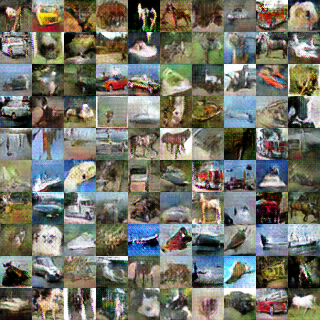
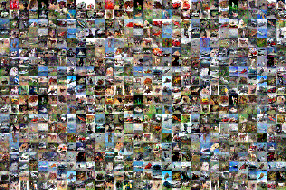
The image is generated by the generator trained for 1000 epochs, and the GIF image
on the top of this page shows generated images after every 10 epochs.
