MNIST using Trainer¶

In the example code of this tutorial, we assume for simplicity that the following symbols are already imported.

import math
import numpy as np
import chainer
from chainer import backend
from chainer import backends
from chainer.backends import cuda
from chainer import Function, FunctionNode, gradient_check, report, training, utils, Variable
from chainer import datasets, initializers, iterators, optimizers, serializers
from chainer import Link, Chain, ChainList
import chainer.functions as F
import chainer.links as L
from chainer.training import extensions

By using Trainer, you don’t need to write the training loop explicitly any more. Furthermore, Chainer provides many useful extensions that can be used with Trainer to visualize your results, evaluate your model, store and manage log files more easily.

This example will show how to use the Trainer to train a fully-connected feed-forward neural network on the MNIST dataset.

Note

If you would like to know how to write a training loop without using the Trainer, please check MNIST with a Manual Training Loop instead of this tutorial.

1. Prepare the dataset¶

Load the MNIST dataset, which contains a training set of images and class labels as well as a corresponding test set.

from chainer.datasets import mnist

train, test = mnist.get_mnist()

Note

You can use a Python list as a dataset. That’s because Iterator can take any object as a dataset whose elements can be accessed via [] accessor and whose length can be obtained with len() function. For example,

train = [(x1, t1), (x2, t2), ...]

a list of tuples like this can be used as a dataset.

There are many utility dataset classes defined in datasets. It’s recommended to utilize them in the actual applications.

For example, if your dataset consists of a number of image files, it would take a large amount of memory to load those data into a list like above. In that case, you can use ImageDataset, which just keeps the paths to image files. The actual image data will be loaded from the disk when the corresponding element is requested via [] accessor. Until then, no images are loaded to the memory to reduce memory use.

2. Prepare the dataset iterations¶

Iterator creates a mini-batch from the given dataset.

batchsize = 128

train_iter = iterators.SerialIterator(train, batchsize)
test_iter = iterators.SerialIterator(test, batchsize, False, False)

3. Prepare the model¶

Here, we are going to use the same model as the one defined in MNIST with a Manual Training Loop.

class MLP(Chain):

    def __init__(self, n_mid_units=100, n_out=10):
        super(MLP, self).__init__()
        with self.init_scope():
            self.l1 = L.Linear(None, n_mid_units)
            self.l2 = L.Linear(None, n_mid_units)
            self.l3 = L.Linear(None, n_out)

    def forward(self, x):
        h1 = F.relu(self.l1(x))
        h2 = F.relu(self.l2(h1))
        return self.l3(h2)

gpu_id = 0  # Set to -1 if you use CPU

model = MLP()
if gpu_id >= 0:
    model.to_gpu(gpu_id)

4. Prepare the Updater¶

Trainer is a class that holds all of the necessary components needed for training. The main components are shown below.

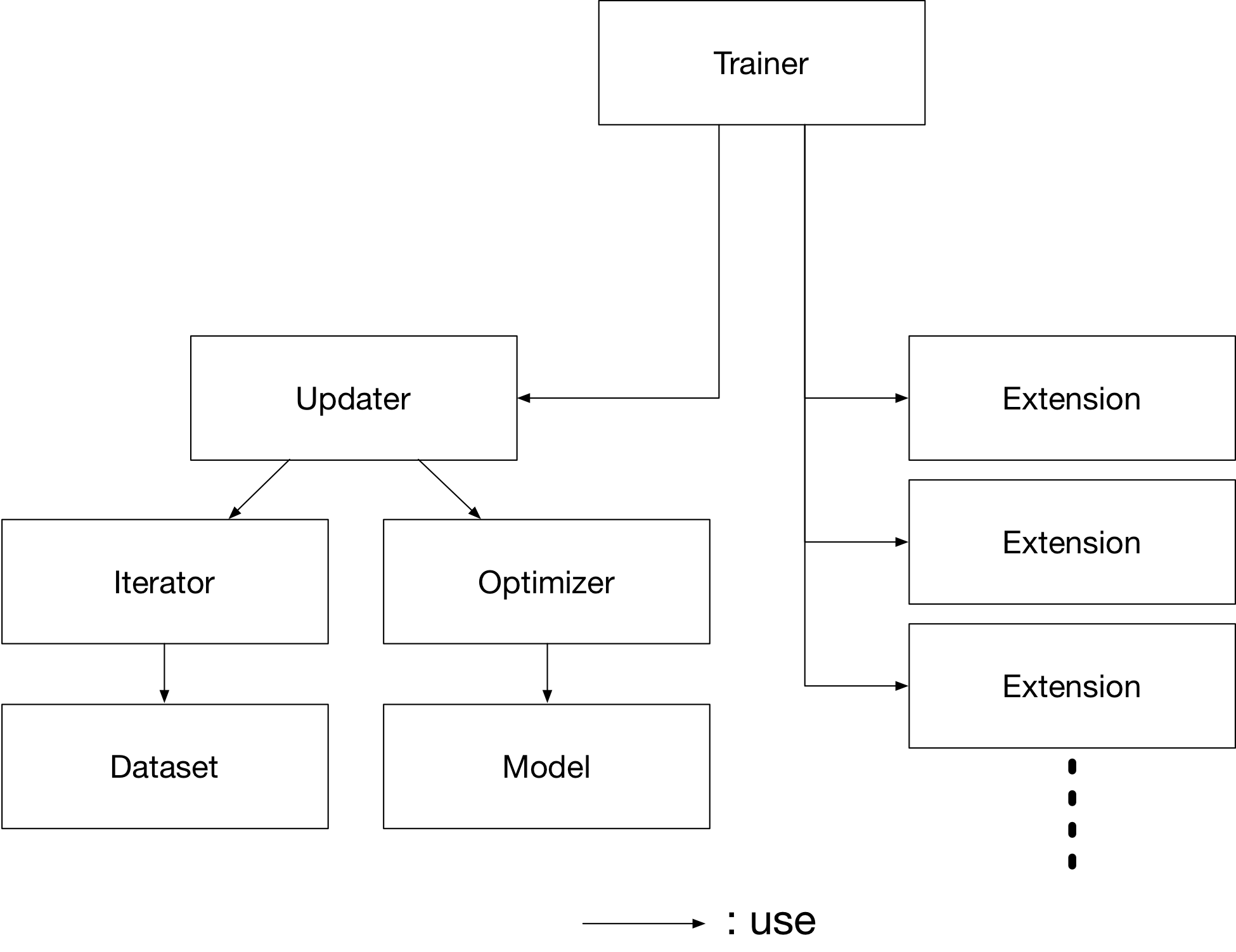
Basically, all you need to pass to Trainer is an Updater. However, Updater contains an Iterator and Optimizer. Since Iterator can access the dataset and Optimizer has references to the model, Updater can access to the model to update its parameters.

So, Updater can perform the training procedure as shown below:

Retrieve the data from dataset and construct a mini-batch (Iterator)
Pass the mini-batch to the model and calculate the loss
Update the parameters of the model (Optimizer)

Now let’s create the Updater object !

max_epoch = 10

# Wrap your model by Classifier and include the process of loss calculation within your model.
# Since we do not specify a loss function here, the default 'softmax_cross_entropy' is used.
model = L.Classifier(model)

# selection of your optimizing method
optimizer = optimizers.MomentumSGD()

# Give the optimizer a reference to the model
optimizer.setup(model)

# Get an updater that uses the Iterator and Optimizer
updater = training.updaters.StandardUpdater(train_iter, optimizer, device=gpu_id)

Note

Here, the model defined above is passed to Classifier and changed to a new Chain. Classifier, which in fact inherits from the Chain class, keeps the given Chain model in its predictor attribute. Once you give the input data and the corresponding class labels to the model by the () operator,

forward() of the model is invoked. The data is then given to predictor to obtain the output y.
Next, together with the given labels, the output y is passed to the loss function which is determined by lossfun argument in the constructor of Classifier.
The loss is returned as a Variable.

In Classifier, the lossfun is set to softmax_cross_entropy() as default.

StandardUpdater is the simplest class among several updaters. There are also the ParallelUpdater and the MultiprocessParallelUpdater to utilize multiple GPUs. The MultiprocessParallelUpdater uses the NVIDIA NCCL library, so you need to install NCCL and re-install CuPy before using it.

5. Setup Trainer¶

Lastly, we will setup Trainer. The only requirement for creating a Trainer is to pass the Updater object that we previously created above. You can also pass a stop_trigger to the second trainer argument as a tuple like (length, unit) to tell the trainer when to stop the training. The length is given as an integer and the unit is given as a string which should be either epoch or iteration. Without setting stop_trigger, the training will never be stopped.

# Setup a Trainer
trainer = training.Trainer(updater, (max_epoch, 'epoch'), out='mnist_result')

The out argument specifies an output directory used to save the log files, the image files of plots to show the time progress of loss, accuracy, etc. when you use PlotReport extension. Next, we will explain how to display or save those information by using trainer Extension.

6. Add Extensions to the Trainer object¶

The Trainer extensions provide the following capabilities:

Save log files automatically (LogReport)
Display the training information to the terminal periodically (PrintReport)
Visualize the loss progress by plotting a graph periodically and save it as an image file (PlotReport)
Automatically serialize the state periodically (snapshot() / snapshot_object())
Display a progress bar to the terminal to show the progress of training (ProgressBar)
Save the model architecture as a Graphviz’s dot file (dump_graph())

To use these wide variety of tools for your training task, pass Extension objects to the extend() method of your Trainer object.

from chainer.training import extensions

trainer.extend(extensions.LogReport())
trainer.extend(extensions.snapshot(filename='snapshot_epoch-{.updater.epoch}'))
trainer.extend(extensions.snapshot_object(model.predictor, filename='model_epoch-{.updater.epoch}'))
trainer.extend(extensions.Evaluator(test_iter, model, device=gpu_id))
trainer.extend(extensions.PrintReport(['epoch', 'main/loss', 'main/accuracy', 'validation/main/loss', 'validation/main/accuracy', 'elapsed_time']))
trainer.extend(extensions.PlotReport(['main/loss', 'validation/main/loss'], x_key='epoch', file_name='loss.png'))
trainer.extend(extensions.PlotReport(['main/accuracy', 'validation/main/accuracy'], x_key='epoch', file_name='accuracy.png'))
trainer.extend(extensions.dump_graph('main/loss'))

`LogReport`¶

Collect loss and accuracy automatically every epoch or iteration and store the information under the log file in the directory specified by the out argument when you create a Trainer object.

`snapshot()`¶

The snapshot() method saves the Trainer object at the designated timing (default: every epoch) in the directory specified by out. The Trainer object, as mentioned before, has an Updater which contains an Optimizer and a model inside. Therefore, as long as you have the snapshot file, you can use it to come back to the training or make inferences using the previously trained model later.

`snapshot_object()`¶

However, when you keep the whole Trainer object, in some cases, it is very tedious to retrieve only the inside of the model. By using snapshot_object(), you can save the particular object (in this case, the model wrapped by Classifier) as a separate snapshot. Classifier is a Chain object which keeps the model that is also a Chain object as its predictor property, and all the parameters are under the predictor, so taking the snapshot of predictor is enough to keep all the trained parameters.

This is a list of commonly used trainer extensions:

LogReport: This extension collects the loss and accuracy values every epoch or iteration and stores in a log file. The log file will be located under the output directory (specified by out argument of the Trainer object).
snapshot(): This extension saves the Trainer object at the designated timing (defaut: every epoch) in the output directory. The Trainer object, as mentioned before, has an Updater which contains an Optimizer and a model inside. Therefore, as long as you have the snapshot file, you can use it to come back to the training or make inferences using the previously trained model later.
snapshot_object(): snapshot() extension above saves the whole Trainer object. However, in some cases, it is tedious to retrieve only the inside of the model. By using snapshot_object(), you can save the particular object (in the example above, the model wrapped by Classifier) as a separeted snapshot. Taking the snapshot of predictor is enough to keep all the trained parameters, because Classifier (which is a subclass of Chain) keeps the model as its predictor property, and all the parameters are under this property.
dump_graph(): This extension saves the structure of the computational graph of the model. The graph is saved in Graphviz dot format under the output directory of the Trainer.
Evaluator: Iterators that use the evaluation dataset and the model object are required to use Evaluator extension. It evaluates the model using the given dataset (typically it’s a validation dataset) at the specified timing interval.
PrintReport: This extension outputs the spcified values to the standard output.
PlotReport: This extension plots the values specified by its arguments and saves it as a image file.

This is not an exhaustive list of built-in extensions. Please take a look at Extensions for more of them.

7. Start Training¶

Just call run() method from Trainer object to start training.

trainer.run()

epoch       main/loss   main/accuracy  validation/main/loss  validation/main/accuracy  elapsed_time
         1.53241     0.638409       0.74935               0.835839                  4.93409
         0.578334    0.858059       0.444722              0.882812                  7.72883
         0.418569    0.886844       0.364943              0.899229                  10.4229
         0.362342    0.899089       0.327569              0.905558                  13.148
         0.331067    0.906517       0.304399              0.911788                  15.846
         0.309019    0.911964       0.288295              0.917722                  18.5395
         0.292312    0.916128       0.272073              0.921776                  21.2173
         0.278291    0.92059        0.261351              0.923457                  23.9211
         0.266266    0.923541       0.253195              0.927314                  26.6612
        0.255489    0.926739       0.242415              0.929094                  29.466

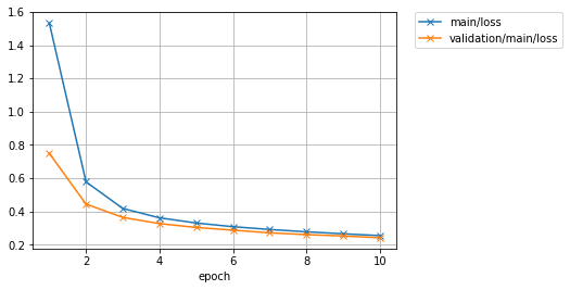
Let’s see the plot of loss progress saved in the mnist_result directory.

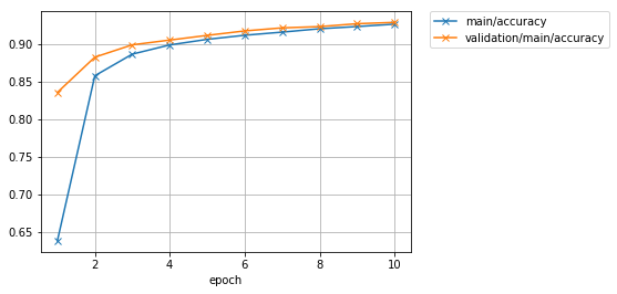
How about the accuracy?

Furthermore, let’s visualize the computational graph saved with dump_graph() using Graphviz.

% dot -Tpng mnist_result/cg.dot -o mnist_result/cg.png

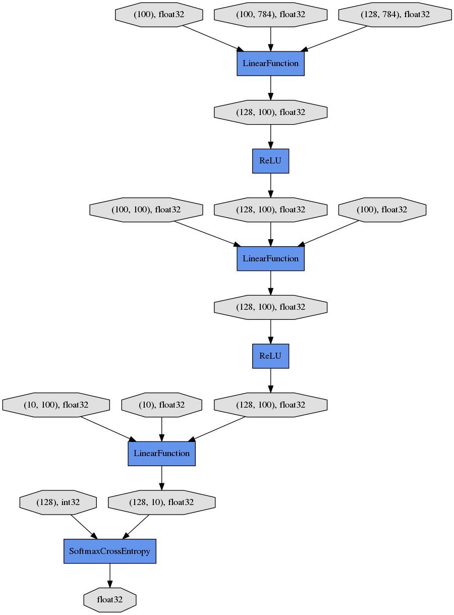
From the top to the bottom, you can see the data flow in the computational graph. It basically shows how data and parameters are passed to the Functions.

8. Evaluate a pre-trained model¶

Evaluation using the snapshot of a model is as easy as what explained in the MNIST with a Manual Training Loop.

import matplotlib.pyplot as plt

model = MLP()
serializers.load_npz('mnist_result/model_epoch-10', model)

# Show the output
x, t = test[0]
plt.imshow(x.reshape(28, 28), cmap='gray')
plt.show()
print('label:', t)

y = model(x[None, ...])

print('predicted_label:', y.array.argmax(axis=1)[0])

label: 7
predicted_label: 7

The prediction looks correct. Success!

MNIST using Trainer¶

1. Prepare the dataset¶

2. Prepare the dataset iterations¶

3. Prepare the model¶

4. Prepare the Updater¶

5. Setup Trainer¶

6. Add Extensions to the Trainer object¶

LogReport¶

snapshot()¶

snapshot_object()¶

7. Start Training¶

8. Evaluate a pre-trained model¶

`LogReport`¶

`snapshot()`¶

`snapshot_object()`¶