librosa.segment.agglomerative

librosa.segment.agglomerative(data, k, clusterer=None, axis=-1)

Bottom-up temporal segmentation.

Use a temporally-constrained agglomerative clustering routine to partition data into k contiguous segments.

Parameters:

data : np.ndarray

data to cluster

k : int > 0 [scalar]

number of segments to produce

clusterer : sklearn.cluster.AgglomerativeClustering, optional

An optional AgglomerativeClustering object. If None, a constrained Ward object is instantiated.

axis : int

axis along which to cluster. By default, the last axis (-1) is chosen.

Returns:

boundaries : np.ndarray [shape=(k,)]

left-boundaries (frame numbers) of detected segments. This will always include 0 as the first left-boundary.

See also

sklearn.cluster.AgglomerativeClustering

Examples

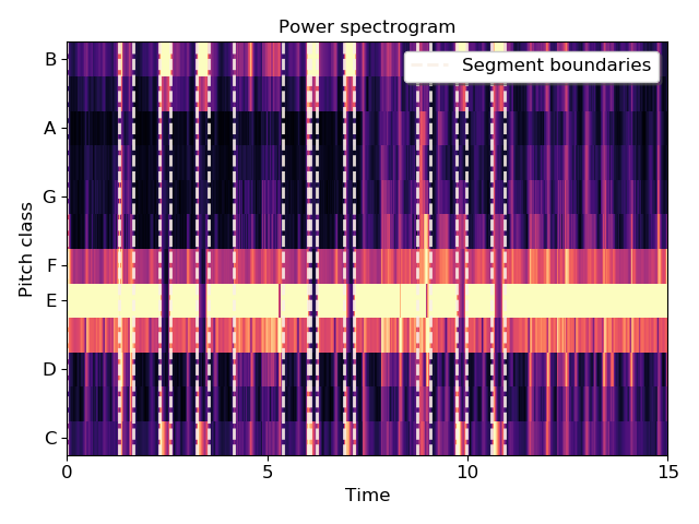
Cluster by chroma similarity, break into 20 segments

>>> y, sr = librosa.load(librosa.util.example_audio_file(), duration=15)
>>> chroma = librosa.feature.chroma_cqt(y=y, sr=sr)
>>> bounds = librosa.segment.agglomerative(chroma, 20)
>>> bound_times = librosa.frames_to_time(bounds, sr=sr)
>>> bound_times
array([  0.   ,   1.672,   2.322,   2.624,   3.251,   3.506,
         4.18 ,   5.387,   6.014,   6.293,   6.943,   7.198,
         7.848,   9.033,   9.706,   9.961,  10.635,  10.89 ,
        11.54 ,  12.539])

Plot the segmentation over the chromagram

>>> import matplotlib.pyplot as plt
>>> plt.figure()
>>> librosa.display.specshow(chroma, y_axis='chroma', x_axis='time')
>>> plt.vlines(bound_times, 0, chroma.shape[0], color='linen', linestyle='--',
...            linewidth=2, alpha=0.9, label='Segment boundaries')
>>> plt.axis('tight')
>>> plt.legend(frameon=True, shadow=True)
>>> plt.title('Power spectrogram')
>>> plt.tight_layout()

(Source code)