librosa.core.fmt

librosa.core.fmt(y, t_min=0.5, n_fmt=None, kind=’cubic’, beta=0.5, over_sample=1, axis=-1)

The fast Mellin transform (FMT) [1] of a uniformly sampled signal y.

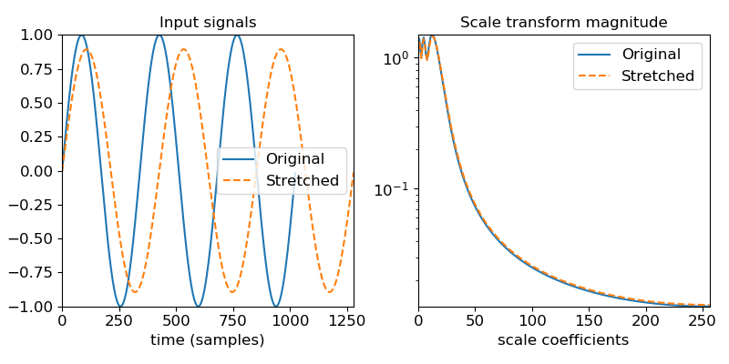
When the Mellin parameter (beta) is 1/2, it is also known as the scale transform [2]. The scale transform can be useful for audio analysis because its magnitude is invariant to scaling of the domain (e.g., time stretching or compression). This is analogous to the magnitude of the Fourier transform being invariant to shifts in the input domain.

[1]	De Sena, Antonio, and Davide Rocchesso. “A fast Mellin and scale transform.” EURASIP Journal on Applied Signal Processing 2007.1 (2007): 75-75.

[2]	Cohen, L. “The scale representation.” IEEE Transactions on Signal Processing 41, no. 12 (1993): 3275-3292.

Parameters:

y : np.ndarray, real-valued

The input signal(s). Can be multidimensional. The target axis must contain at least 3 samples.

t_min : float > 0

The minimum time spacing (in samples). This value should generally be less than 1 to preserve as much information as possible.

n_fmt : int > 2 or None

The number of scale transform bins to use. If None, then n_bins = over_sample * ceil(n * log((n-1)/t_min)) is taken, where n = y.shape[axis]

kind : str

The type of interpolation to use when re-sampling the input. See scipy.interpolate.interp1d for possible values.

Note that the default is to use high-precision (cubic) interpolation. This can be slow in practice; if speed is preferred over accuracy, then consider using kind=’linear’.

beta : float

The Mellin parameter. beta=0.5 provides the scale transform.

over_sample : float >= 1

Over-sampling factor for exponential resampling.

axis : int

The axis along which to transform y

Returns:

x_scale : np.ndarray [dtype=complex]

The scale transform of y along the axis dimension.

Raises:

ParameterError

if n_fmt < 2 or t_min <= 0 or if y is not finite or if y.shape[axis] < 3.

Notes

This function caches at level 30.

Examples

>>> # Generate a signal and time-stretch it (with energy normalization)
>>> scale = 1.25
>>> freq = 3.0
>>> x1 = np.linspace(0, 1, num=1024, endpoint=False)
>>> x2 = np.linspace(0, 1, num=scale * len(x1), endpoint=False)
>>> y1 = np.sin(2 * np.pi * freq * x1)
>>> y2 = np.sin(2 * np.pi * freq * x2) / np.sqrt(scale)
>>> # Verify that the two signals have the same energy
>>> np.sum(np.abs(y1)**2), np.sum(np.abs(y2)**2)
    (255.99999999999997, 255.99999999999969)
>>> scale1 = librosa.fmt(y1, n_fmt=512)
>>> scale2 = librosa.fmt(y2, n_fmt=512)
>>> # And plot the results
>>> import matplotlib.pyplot as plt
>>> plt.figure(figsize=(8, 4))
>>> plt.subplot(1, 2, 1)
>>> plt.plot(y1, label='Original')
>>> plt.plot(y2, linestyle='--', label='Stretched')
>>> plt.xlabel('time (samples)')
>>> plt.title('Input signals')
>>> plt.legend(frameon=True)
>>> plt.axis('tight')
>>> plt.subplot(1, 2, 2)
>>> plt.semilogy(np.abs(scale1), label='Original')
>>> plt.semilogy(np.abs(scale2), linestyle='--', label='Stretched')
>>> plt.xlabel('scale coefficients')
>>> plt.title('Scale transform magnitude')
>>> plt.legend(frameon=True)
>>> plt.axis('tight')
>>> plt.tight_layout()

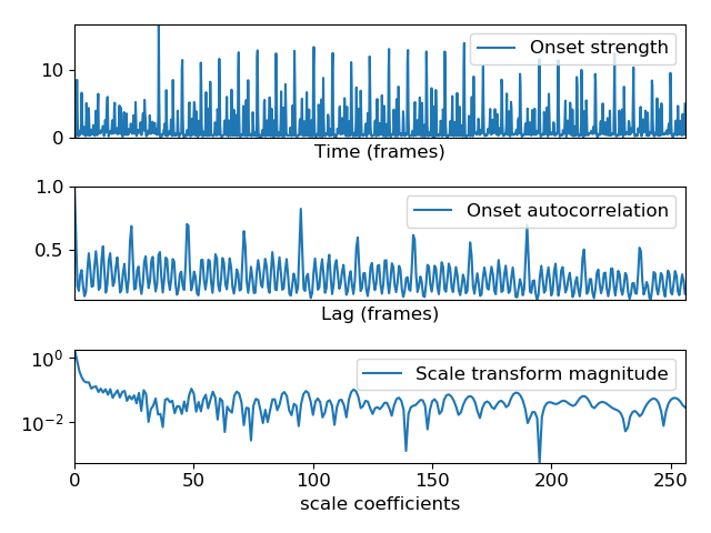
>>> # Plot the scale transform of an onset strength autocorrelation
>>> y, sr = librosa.load(librosa.util.example_audio_file(),
...                      offset=10.0, duration=30.0)
>>> odf = librosa.onset.onset_strength(y=y, sr=sr)
>>> # Auto-correlate with up to 10 seconds lag
>>> odf_ac = librosa.autocorrelate(odf, max_size=10 * sr // 512)
>>> # Normalize
>>> odf_ac = librosa.util.normalize(odf_ac, norm=np.inf)
>>> # Compute the scale transform
>>> odf_ac_scale = librosa.fmt(librosa.util.normalize(odf_ac), n_fmt=512)
>>> # Plot the results
>>> plt.figure()
>>> plt.subplot(3, 1, 1)
>>> plt.plot(odf, label='Onset strength')
>>> plt.axis('tight')
>>> plt.xlabel('Time (frames)')
>>> plt.xticks([])
>>> plt.legend(frameon=True)
>>> plt.subplot(3, 1, 2)
>>> plt.plot(odf_ac, label='Onset autocorrelation')
>>> plt.axis('tight')
>>> plt.xlabel('Lag (frames)')
>>> plt.xticks([])
>>> plt.legend(frameon=True)
>>> plt.subplot(3, 1, 3)
>>> plt.semilogy(np.abs(odf_ac_scale), label='Scale transform magnitude')
>>> plt.axis('tight')
>>> plt.xlabel('scale coefficients')
>>> plt.legend(frameon=True)
>>> plt.tight_layout()

(Source code)