Graph Structures
Theano Graphs
Debugging or profiling code written in Theano is not that simple if you do not know what goes on under the hood. This chapter is meant to introduce you to a required minimum of the inner workings of Theano. For more detail see Extending Theano.
The first step in writing Theano code is to write down all mathematical
relations using symbolic placeholders (variables). When writing down
these expressions you use operations like +, -, **,
sum(), tanh(). All these are represented internally as ops.
An op represents a certain computation on some type of inputs
producing some type of output. You can see it as a function definition
in most programming languages.
Theano builds internally a graph structure composed of interconnected variable nodes, op nodes and apply nodes. An apply node represents the application of an op to some variables. It is important to draw the difference between the definition of a computation represented by an op and its application to some actual data which is represented by the apply node. For more detail about these building blocks refer to Variable, Op, Apply. Here is an example of a graph:
Code
import theano.tensor as T
x = T.dmatrix('x')
y = T.dmatrix('y')
z = x + y
Diagram
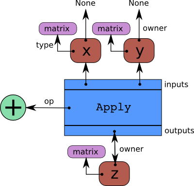
Interaction between instances of Apply (blue), Variable (red), Op (green), and Type (purple).
Arrows in this figure represent references to the Python objects pointed at. The blue box is an Apply node. Red boxes are Variable nodes. Green circles are Ops. Purple boxes are Types.
The graph can be traversed starting from outputs (the result of some computation) down to its inputs using the owner field. Take for example the following code:
>>> import theano
>>> x = theano.tensor.dmatrix('x')
>>> y = x * 2.
If you enter type(y.owner) you get <class 'theano.gof.graph.Apply'>,
which is the apply node that connects the op and the inputs to get this
output. You can now print the name of the op that is applied to get
y:
>>> y.owner.op.name
'Elemwise{mul,no_inplace}'
Hence, an elementwise multiplication is used to compute y. This multiplication is done between the inputs:
>>> len(y.owner.inputs)
2
>>> y.owner.inputs[0]
x
>>> y.owner.inputs[1]
DimShuffle{x,x}.0
Note that the second input is not 2 as we would have expected. This is
because 2 was first broadcasted to a matrix of
same shape as x. This is done by using the op DimShuffle :
>>> type(y.owner.inputs[1])
<class 'theano.tensor.var.TensorVariable'>
>>> type(y.owner.inputs[1].owner)
<class 'theano.gof.graph.Apply'>
>>> y.owner.inputs[1].owner.op
<theano.tensor.elemwise.DimShuffle object at 0x106fcaf10>
>>> y.owner.inputs[1].owner.inputs
[TensorConstant{2.0}]
Starting from this graph structure it is easier to understand how automatic differentiation proceeds and how the symbolic relations can be optimized for performance or stability.
Automatic Differentiation
Having the graph structure, computing automatic differentiation is
simple. The only thing tensor.grad() has to do is to traverse the
graph from the outputs back towards the inputs through all apply
nodes (apply nodes are those that define which computations the
graph does). For each such apply node, its op defines
how to compute the gradient of the node’s outputs with respect to its
inputs. Note that if an op does not provide this information,
it is assumed that the gradient is not defined.
Using the
chain rule
these gradients can be composed in order to obtain the expression of the
gradient of the graph’s output with respect to the graph’s inputs .
A following section of this tutorial will examine the topic of differentiation in greater detail.
Optimizations
When compiling a Theano function, what you give to the
theano.function is actually a graph
(starting from the output variables you can traverse the graph up to
the input variables). While this graph structure shows how to compute
the output from the input, it also offers the possibility to improve the
way this computation is carried out. The way optimizations work in
Theano is by identifying and replacing certain patterns in the graph
with other specialized patterns that produce the same results but are either
faster or more stable. Optimizations can also detect
identical subgraphs and ensure that the same values are not computed
twice or reformulate parts of the graph to a GPU specific version.
For example, one (simple) optimization that Theano uses is to replace
the pattern  by x.
by x.
Further information regarding the optimization process and the specific optimizations that are applicable is respectively available in the library and on the entrance page of the documentation.
Example
Symbolic programming involves a change of paradigm: it will become clearer as we apply it. Consider the following example of optimization:
>>> import theano
>>> a = theano.tensor.vector("a")      # declare symbolic variable
>>> b = a + a ** 10                    # build symbolic expression
>>> f = theano.function([a], b)        # compile function
>>> print f([0, 1, 2])                 # prints `array([0,2,1026])`
[    0.     2.  1026.]
>>> theano.printing.pydotprint(b, outfile="./pics/symbolic_graph_unopt.png", var_with_name_simple=True)
The output file is available at ./pics/symbolic_graph_unopt.png
>>> theano.printing.pydotprint(f, outfile="./pics/symbolic_graph_opt.png", var_with_name_simple=True)
The output file is available at ./pics/symbolic_graph_opt.png
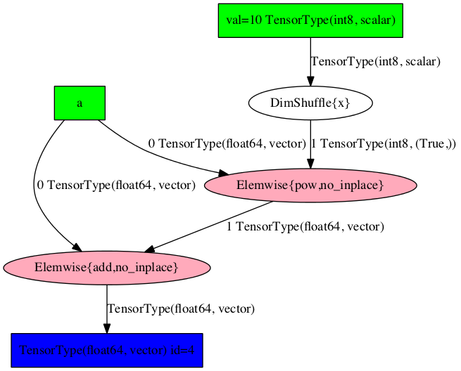
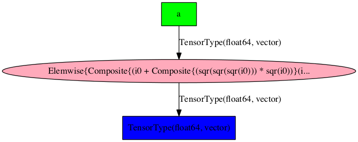
We used theano.printing.pydotprint() to visualize the optimized graph
(right), which is much more compact than the unoptimized graph (left).
| Unoptimized graph | Optimized graph |
|---|---|
 |
 |