librosa.feature.tonnetz

librosa.feature.tonnetz(y=None, sr=22050, chroma=None)

Computes the tonal centroid features (tonnetz), following the method of [1].

[1]	Harte, C., Sandler, M., & Gasser, M. (2006). “Detecting Harmonic Change in Musical Audio.” In Proceedings of the 1st ACM Workshop on Audio and Music Computing Multimedia (pp. 21-26). Santa Barbara, CA, USA: ACM Press. doi:10.1145/1178723.1178727.

Parameters:

y : np.ndarray [shape=(n,)] or None

Audio time series.

sr : number > 0 [scalar]

sampling rate of y

chroma : np.ndarray [shape=(n_chroma, t)] or None

Normalized energy for each chroma bin at each frame.

If None, a cqt chromagram is performed.

Returns:

tonnetz : np.ndarray [shape(6, t)]

Tonal centroid features for each frame.

Tonnetz dimensions:

• 0: Fifth x-axis
• 1: Fifth y-axis
• 2: Minor x-axis
• 3: Minor y-axis
• 4: Major x-axis
• 5: Major y-axis

See also

chroma_cqt

Compute a chromagram from a constant-Q transform.

chroma_stft

Compute a chromagram from an STFT spectrogram or waveform.

Examples

Compute tonnetz features from the harmonic component of a song

>>> y, sr = librosa.load(librosa.util.example_audio_file())
>>> y = librosa.effects.harmonic(y)
>>> tonnetz = librosa.feature.tonnetz(y=y, sr=sr)
>>> tonnetz
array([[-0.073, -0.053, ..., -0.054, -0.073],
       [ 0.001,  0.001, ..., -0.054, -0.062],
       ...,
       [ 0.039,  0.034, ...,  0.044,  0.064],
       [ 0.005,  0.002, ...,  0.011,  0.017]])

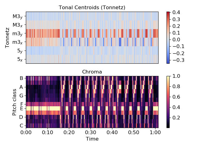
Compare the tonnetz features to chroma_cqt

>>> import matplotlib.pyplot as plt
>>> plt.subplot(2, 1, 1)
>>> librosa.display.specshow(tonnetz, y_axis='tonnetz')
>>> plt.colorbar()
>>> plt.title('Tonal Centroids (Tonnetz)')
>>> plt.subplot(2, 1, 2)
>>> librosa.display.specshow(librosa.feature.chroma_cqt(y, sr=sr),
...                          y_axis='chroma', x_axis='time')
>>> plt.colorbar()
>>> plt.title('Chroma')
>>> plt.tight_layout()

(Source code)