librosa.feature.poly_features

librosa.feature.poly_features(y=None, sr=22050, S=None, n_fft=2048, hop_length=512, order=1, freq=None)

Get coefficients of fitting an nth-order polynomial to the columns of a spectrogram.

Parameters:

y : np.ndarray [shape=(n,)] or None

audio time series

sr : number > 0 [scalar]

audio sampling rate of y

S : np.ndarray [shape=(d, t)] or None

(optional) spectrogram magnitude

n_fft : int > 0 [scalar]

FFT window size

hop_length : int > 0 [scalar]

hop length for STFT. See librosa.core.stft for details.

order : int > 0

order of the polynomial to fit

freq : None or np.ndarray [shape=(d,) or shape=(d, t)]

Center frequencies for spectrogram bins. If None, then FFT bin center frequencies are used. Otherwise, it can be a single array of d center frequencies, or a matrix of center frequencies as constructed by librosa.core.ifgram

Returns:

coefficients : np.ndarray [shape=(order+1, t)]

polynomial coefficients for each frame.

coeffecients[0] corresponds to the highest degree (order),

coefficients[1] corresponds to the next highest degree (order-1),

down to the constant term coefficients[order].

Examples

>>> y, sr = librosa.load(librosa.util.example_audio_file())
>>> S = np.abs(librosa.stft(y))

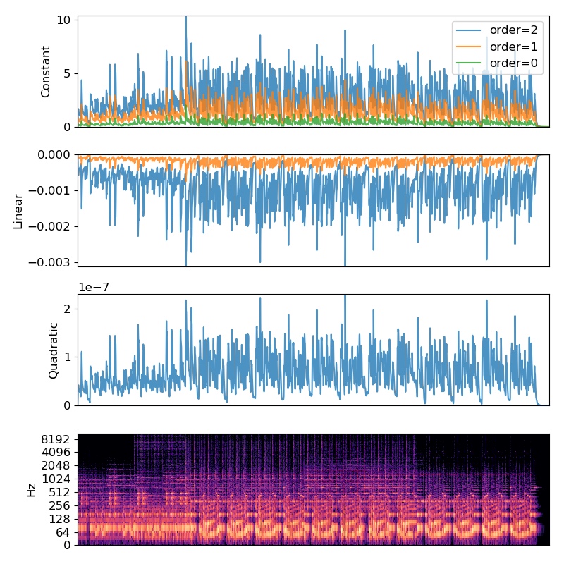
Fit a degree-0 polynomial (constant) to each frame

>>> p0 = librosa.feature.poly_features(S=S, order=0)

Fit a linear polynomial to each frame

>>> p1 = librosa.feature.poly_features(S=S, order=1)

Fit a quadratic to each frame

>>> p2 = librosa.feature.poly_features(S=S, order=2)

Plot the results for comparison

>>> import matplotlib.pyplot as plt
>>> plt.figure(figsize=(8, 8))
>>> ax = plt.subplot(4,1,1)
>>> plt.plot(p2[2], label='order=2', alpha=0.8)
>>> plt.plot(p1[1], label='order=1', alpha=0.8)
>>> plt.plot(p0[0], label='order=0', alpha=0.8)
>>> plt.xticks([])
>>> plt.ylabel('Constant')
>>> plt.legend()
>>> plt.subplot(4,1,2, sharex=ax)
>>> plt.plot(p2[1], label='order=2', alpha=0.8)
>>> plt.plot(p1[0], label='order=1', alpha=0.8)
>>> plt.xticks([])
>>> plt.ylabel('Linear')
>>> plt.subplot(4,1,3, sharex=ax)
>>> plt.plot(p2[0], label='order=2', alpha=0.8)
>>> plt.xticks([])
>>> plt.ylabel('Quadratic')
>>> plt.subplot(4,1,4, sharex=ax)
>>> librosa.display.specshow(librosa.amplitude_to_db(S, ref=np.max),
...                          y_axis='log')
>>> plt.tight_layout()

(Source code)