librosa.feature.spectral_centroid

librosa.feature.spectral_centroid(y=None, sr=22050, S=None, n_fft=2048, hop_length=512, freq=None)

Compute the spectral centroid.

Each frame of a magnitude spectrogram is normalized and treated as a distribution over frequency bins, from which the mean (centroid) is extracted per frame.

Parameters:

y : np.ndarray [shape=(n,)] or None

audio time series

sr : number > 0 [scalar]

audio sampling rate of y

S : np.ndarray [shape=(d, t)] or None

(optional) spectrogram magnitude

n_fft : int > 0 [scalar]

FFT window size

hop_length : int > 0 [scalar]

hop length for STFT. See librosa.core.stft for details.

freq : None or np.ndarray [shape=(d,) or shape=(d, t)]

Center frequencies for spectrogram bins. If None, then FFT bin center frequencies are used. Otherwise, it can be a single array of d center frequencies, or a matrix of center frequencies as constructed by librosa.core.ifgram

Returns:

centroid : np.ndarray [shape=(1, t)]

centroid frequencies

See also

librosa.core.stft

Short-time Fourier Transform

librosa.core.ifgram

Instantaneous-frequency spectrogram

Examples

From time-series input:

>>> y, sr = librosa.load(librosa.util.example_audio_file())
>>> cent = librosa.feature.spectral_centroid(y=y, sr=sr)
>>> cent
array([[ 4382.894,   626.588, ...,  5037.07 ,  5413.398]])

From spectrogram input:

>>> S, phase = librosa.magphase(librosa.stft(y=y))
>>> librosa.feature.spectral_centroid(S=S)
array([[ 4382.894,   626.588, ...,  5037.07 ,  5413.398]])

Using variable bin center frequencies:

>>> y, sr = librosa.load(librosa.util.example_audio_file())
>>> if_gram, D = librosa.ifgram(y)
>>> librosa.feature.spectral_centroid(S=np.abs(D), freq=if_gram)
array([[ 4420.719,   625.769, ...,  5011.86 ,  5221.492]])

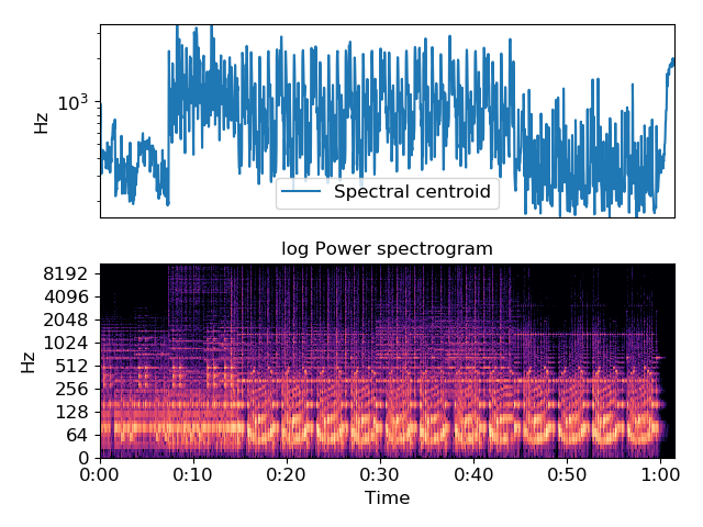
Plot the result

>>> import matplotlib.pyplot as plt
>>> plt.figure()
>>> plt.subplot(2, 1, 1)
>>> plt.semilogy(cent.T, label='Spectral centroid')
>>> plt.ylabel('Hz')
>>> plt.xticks([])
>>> plt.xlim([0, cent.shape[-1]])
>>> plt.legend()
>>> plt.subplot(2, 1, 2)
>>> librosa.display.specshow(librosa.amplitude_to_db(S, ref=np.max),
...                          y_axis='log', x_axis='time')
>>> plt.title('log Power spectrogram')
>>> plt.tight_layout()

(Source code)