librosa.feature.melspectrogram

librosa.feature.melspectrogram(y=None, sr=22050, S=None, n_fft=2048, hop_length=512, power=2.0, **kwargs)

Compute a mel-scaled spectrogram.

If a spectrogram input S is provided, then it is mapped directly onto the mel basis mel_f by mel_f.dot(S).

If a time-series input y, sr is provided, then its magnitude spectrogram S is first computed, and then mapped onto the mel scale by mel_f.dot(S**power). By default, power=2 operates on a power spectrum.

Parameters:

y : np.ndarray [shape=(n,)] or None

audio time-series

sr : number > 0 [scalar]

sampling rate of y

S : np.ndarray [shape=(d, t)]

spectrogram

n_fft : int > 0 [scalar]

length of the FFT window

hop_length : int > 0 [scalar]

number of samples between successive frames. See librosa.core.stft

power : float > 0 [scalar]

Exponent for the magnitude melspectrogram. e.g., 1 for energy, 2 for power, etc.

kwargs : additional keyword arguments

Mel filter bank parameters. See librosa.filters.mel for details.

Returns:

S : np.ndarray [shape=(n_mels, t)]

Mel spectrogram

See also

librosa.filters.mel

Mel filter bank construction

librosa.core.stft

Short-time Fourier Transform

Examples

>>> y, sr = librosa.load(librosa.util.example_audio_file())
>>> librosa.feature.melspectrogram(y=y, sr=sr)
array([[  2.891e-07,   2.548e-03, ...,   8.116e-09,   5.633e-09],
       [  1.986e-07,   1.162e-02, ...,   9.332e-08,   6.716e-09],
       ...,
       [  3.668e-09,   2.029e-08, ...,   3.208e-09,   2.864e-09],
       [  2.561e-10,   2.096e-09, ...,   7.543e-10,   6.101e-10]])

Using a pre-computed power spectrogram

>>> D = np.abs(librosa.stft(y))**2
>>> S = librosa.feature.melspectrogram(S=D)

>>> # Passing through arguments to the Mel filters
>>> S = librosa.feature.melspectrogram(y=y, sr=sr, n_mels=128,
...                                     fmax=8000)

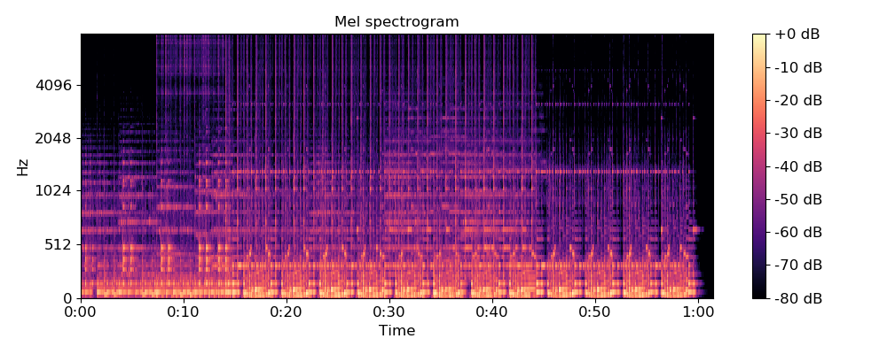
>>> import matplotlib.pyplot as plt
>>> plt.figure(figsize=(10, 4))
>>> librosa.display.specshow(librosa.power_to_db(S,
...                                              ref=np.max),
...                          y_axis='mel', fmax=8000,
...                          x_axis='time')
>>> plt.colorbar(format='%+2.0f dB')
>>> plt.title('Mel spectrogram')
>>> plt.tight_layout()

(Source code)