librosa.feature.spectral_contrast

librosa.feature.spectral_contrast(y=None, sr=22050, S=None, n_fft=2048, hop_length=512, freq=None, fmin=200.0, n_bands=6, quantile=0.02, linear=False)

Compute spectral contrast [1]

[1]	Jiang, Dan-Ning, Lie Lu, Hong-Jiang Zhang, Jian-Hua Tao, and Lian-Hong Cai. “Music type classification by spectral contrast feature.” In Multimedia and Expo, 2002. ICME‘02. Proceedings. 2002 IEEE International Conference on, vol. 1, pp. 113-116. IEEE, 2002.

Parameters:

y : np.ndarray [shape=(n,)] or None

audio time series

sr : number > 0 [scalar]

audio sampling rate of y

S : np.ndarray [shape=(d, t)] or None

(optional) spectrogram magnitude

n_fft : int > 0 [scalar]

FFT window size

hop_length : int > 0 [scalar]

hop length for STFT. See librosa.core.stft for details.

freq : None or np.ndarray [shape=(d,)]

Center frequencies for spectrogram bins. If None, then FFT bin center frequencies are used. Otherwise, it can be a single array of d center frequencies.

fmin : float > 0

Frequency cutoff for the first bin [0, fmin] Subsequent bins will cover [fmin, 2*fmin], [2*fmin, 4*fmin], etc.

n_bands : int > 1

number of frequency bands

quantile : float in (0, 1)

quantile for determining peaks and valleys

linear : bool

If True, return the linear difference of magnitudes: peaks - valleys.

If False, return the logarithmic difference: log(peaks) - log(valleys).

Returns:

contrast : np.ndarray [shape=(n_bands + 1, t)]

each row of spectral contrast values corresponds to a given octave-based frequency

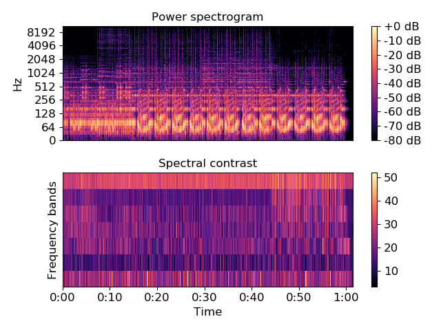
Examples

>>> y, sr = librosa.load(librosa.util.example_audio_file())
>>> S = np.abs(librosa.stft(y))
>>> contrast = librosa.feature.spectral_contrast(S=S, sr=sr)

>>> import matplotlib.pyplot as plt
>>> plt.figure()
>>> plt.subplot(2, 1, 1)
>>> librosa.display.specshow(librosa.amplitude_to_db(S,
...                                                  ref=np.max),
...                          y_axis='log')
>>> plt.colorbar(format='%+2.0f dB')
>>> plt.title('Power spectrogram')
>>> plt.subplot(2, 1, 2)
>>> librosa.display.specshow(contrast, x_axis='time')
>>> plt.colorbar()
>>> plt.ylabel('Frequency bands')
>>> plt.title('Spectral contrast')
>>> plt.tight_layout()

(Source code)